Interval Type-3 Fuzzy Broad Learning System with Its Application in Uncertain System Regression Modeling
Received Date: June 20, 2025 Accepted Date: July 04, 2025 Published Date: July 07, 2025
doi:10.17303/jaist.2025.2.201
Citation: Hao Tian, Jian Tang, Luhong Guo (2025) Interval Type-3 Fuzzy Broad Learning System with Its Application in Uncertain System Regression Modeling.J Artif Intel Sost Comp Tech 2: 1-31
Abstract
Traditional Type-I and Type-2 fuzzy systems face limitations in addressing complex uncertainties. To overcome these challenges, a novel framework integrating the Interval Type-3 Fuzzy System (IT3FS) with a Broad Learning System (BLS) was developed, referred to as the Interval Type-3 Fuzzy Broad Learning System (IT3FBLS). This approach combines the advanced uncertainty representation capabilities of Type-3 fuzzy logic with the computational efficiency of BLS, effectively addressing the modeling difficulties associated with complex, nonlinear, and uncertain data. In the IT3FBIS, an entropy-based adaptive regularization and gradient quadratic optimization strategy is introduced for parameter learning, 'Ibis strategy dynamically adjusts node distribution and feature contribution, thereby improving robustness and generalization in the context of high-dimensional, multi-source heterogeneous data. Modeling experiments were conducted using low-to-medium-dimensional public datasets, uncertain functions, and reaLworld industrial process data, The results, when compared to several conventional and advanced BLS and fuzzy models,
Keywords: Interval Type-3 Fuzzy System (IT3FS); Broad Learning System (BLS); Entropy-Based Parameter Learning; Interval Type-3 Fuzzy BLS (IT3FBLS); Industrial Process Modeling
Introduction
With the rapid development of sensor networks and information technology, industrial production processes are generating vast amounts of multisource heterogeneous data Ill. These data often exhibit prominent non-Gaussian characteristics and dynamic coupling effects 121, while also being influenced by various stochastic factors, resulting in significant uncertainty in both data distribution and system behavior 131. Traditional approaches typically rely on prior assumptions alx»ut system mecha- nisms [41, making them inadequate for capturing the highly nonlinear and multi-layered uncertainties inherent in indus- trial prcxesses. At the same time, the increasing demand for real-time performance and accuracy has highlighted a critical challenge: how to develop regression that can operate efficiently and reliably in high-dimensional, dynam- icy and noisy data environments. This challenge has increas- ingly become a bottleneck in the intelligent transformation of industrial processes [5]. Therefore, the development of more flexible, efficient, and adaptive data-driven modeling theories and methods, capable of handling complex and uncertain datasets, has become a key focus of both academic research and industrial applications.
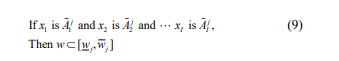
Ami e continuous advancement of industrial big data and artificial intelligence (A1) technologies [6], data-driven modeling strategies are emerging as a powerful solution to the challenges of complex industrial process modeling. Among these, fuzzy logic systems (FLS) [7] have gained widespread adoption in industrial research and optimization due to their ability to handle nonlinear problems without requiring explicit mathematical models. Building on this foundation, fuzzy neural networks (FNN) [8] combine the fuzzy inference and uncertainty-handling capabilities of FLS with the adaptive learning potential of neural networks, enabling automatic parameter adjustment. Applications of FNN in areas such as municipal solid waste incineration (MSWI) and wastewater treatment processes (WWTP) have demonstrated promising results [9,10], highlighting its strong potential for improving process modeling and control.
However, the widely adopted early-generation Type. 1 Fuzzy Systems (Tl FS) exhibit inherent limitations in handling uncertainty, as their memtRrship functions can only depict single-layer fuzzy boundaries, rendering them ineffective in complex environments characterized by severe noise and disturbances [11 To address these shortcomings, reRarchers introduced interval tYF2 fuzzy systems (IT2FS), which can incorporate uncertainty boundaries, thereby significantly expanding the applicability of fuzzy logic in complex and uncertain environments 1121. Leveraging the enhanced uncertainty modeling capabilities of IT2FS, interval type-2 fuzzy neural networks (IT2FNN) have found widespread applications in industrial process control [13].
Despite the significant advancements brought by IT2FS in extending fuzzy boundaries, their secondary mem bership functions are typically confined to interval forms, limiting their capacity to capture multi-level, unstable, or time-varying Ihis limitation becomes particularly pronounced when dealing with non-Gaussian noise and multi-modal fuzzy distributions, leading to potential modeling biases [141. Consequently, improving the adapt. ability of fuzzy systems to handle multi-level uncertainties without significantly increasing system complexity has become a critical direction.
To further enhance the modeling capabilities of fuzzy systems, general type-2 fuzzy systems (GT2FS) were proposed, extending secondary membership functions into Type-I fuzzy sets, thereby theoretically enabling a more precise characterization of high-dimensional uncertainties [15,161. However, the complex structure and substantial computational overhead associated with GT2FS have hindered their practical deployment in industrial scenarios requiring real-time processing 1171. As an improvement, interval type-3 fuzzy systems (IT3FS), based on type-3 FIS (T3FLS), were introduced [18]. These systems utilize interval type-2 fuzzy sets to construct secondary membership functions, effectively balancing the enhanced uncertain. ty.handling capacity of type-3 fuzzy systems with reduced computational complexity. IT3FS has already demonstrated promising potential in nonlinear dynamic system control and predictive modeling[19,20,21]
Nevertheless, while IT3FS represents a significant advance. ment in uncertainty management, its complex system architecture also introduces an expansive parameter space. In practical applications, particularly within adaptive control domains, fuzzy models should satisfy real. time online learning and dynamic updates, The substantial parameter tuning and high-dimensional search requirements of IT3FS not only complicate algorithmic convergence but also impose considerable computational burdens, thereby constraining its feasibility for real-time industrial applications [22]. Therefore, designing more effcient parameter learning algorithms to unlock the full modeling potential of IT3FS, while reducing computational costs, remains an open issue to be solved.
To address the challenges asscxiated with parameter learning in IT3FS, the recently mular broad learning system (BLS) [23] Offers a promising solution. BLS focuses on rapid learning through feature mapping and an enhanced node structure. Unlike conventional deep learning frame. works, BLS eliminates the need for multi-layer iterative training, requiring only output layer weight updates to accomplish large-scale data learning, thus significantly reducing computational complexity [24,25]. Moreover, its parallel computing and incremental learning mechanisms enable more efficient and feasible online updates in dynamic environments. By integrating the advanced uncertainty representation of IT3FS with the efficient learning mechanism of BLS, it becomes feasible to develop a fuzzy system characterized by strong adaptability and rapid convergence under complex uncertain conditions.
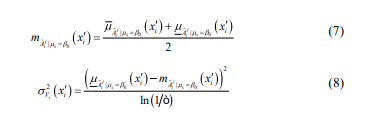
In training regression models for complex datasets, conventional performance evaluation metrics, such as the mean and variance, often fail to fully capture the intricate characteristics of non-Gaussian or multi-mcxial dynamic systems. Entropy, as a critical measure of data diversity, uncertainty, and randomness [26], offers a more effective means of revealing higher-order statistical information. In Inculeling error analysis, lower entropy typically indicates a more concentrated error distribution with reduced volatility, reflecting greater system stability [27]. Therefore, to optimize the parameters of IT3FBIS more precisely, leveraging entropy. based metrics for weight adjustment may enhance the system's adaptability and robustness in uncertain environments.
In summary, to address the challenges of modeling and controlling complex uncertain datasets, this article proposes a novel neural model framework — the interval type-3 fuzzy broad learning system (IT3FBLS) — which integrates IT3FS with BLS. Within this framework, the IT3FS module replaces the feature mapping unit of BLS, retaining the structural simplicity and efficient learning capabilities of BLS while overcoming the high-dimensional parameter learning bottleneck of IT3FS through multi-level uncertainty modeling and rapid learning mechanisms. Additionally, two entropy-based Birameter optimization strategies are introduced, leveraging entropy metrics for model evaluation and adjustment to significantly reduce modeling errors. The effectiveness of the proposed algorithm is ultimately validated through its application in uncertain data regression modeling with different datasets, The primary contributions of this article are as follows:
- To address the challenges of complex uncertainty and real-time regression modeling, an IT3FBLS framework integrating IT3FS and the BLS is proposed. This framework achieves precise regression and adaptive control of complex dynamic systems with high uncertainty capability while requiring only limited training samples.
- By retaining the efficient feature mapping and enhanced node structure of BLS, the IT3FBLS framework further improves modeling performance for high.dimensional and multi-source heterogeneous data. This article also provides an initial exploration of integrating advanced fuzzy logic systems within the BLS framework, offering insights for future advancements in uncertainty modeling.
- Two entropy-weighted secondary parameter optimization algorithms are designed, including an adaptive regularization strategy and a gradient descent-based secondary optimization approach. These algorithms effectively mitigate the impact of random noise and nonstationary disturbances while ensuring dynamic fine-tuning and effective feature extraction, laying the foundation for high-precision regression modeling and robust control.
The remainder of this article is organized as follows: Section 2 introduces the preliminaries, including IT3FS and BLS. Section 3 provides details on the IT3FBIS structure and implementation, entropy-based parameter learning, compu- tational complexity analysis, and algorithm pseudocode. 4 presents experiments and discussions, while Section 5 summarizes the reaserch
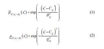
Preliminaries 2.1 Interval Type-3 Fuzzy System (IT3FS)- The IT3FS is a fuzzy logic system designed to handle complex uncertainties. By employing IT2FS to construct secondary memlkrship function (SMF), IT3FS enhances its ability to model uncertainties without signifi- cantly increasing computational complexity. The computa- tional process of IT3FS can be divided into five functional layers: input layer, membership function computation layer, rule inference layer, type-reduction layer, and output layer. The description of each layer is provided in detail as follows. (l) Input layer: The input layer receives external input data and passes it to the membership function computation layer. The system inputs are denoted as where x1,x2,x3,....xn represents the i-th input variable. The primary function of this layer is to prepare and provide input data for subsequent computations.
- Membership function computation layer: The member- ship function computation layer fuzzifiers the input variables by mapping each input xi, to the upper and lower
For the baseline horizontal slice  they are calculated as:
membership degrees of the fuzzy set  The
membership functions are defined based on Gaussian distri-
butions, with the calculations depending on the specific
horizontal slice
The
membership functions are defined based on Gaussian distri-
butions, with the calculations depending on the specific
horizontal slice  when the specific value of input
  the calculation prcxess is as follows.
For the baseline horizontal slice  they are calculated as:
For other horizontal slices 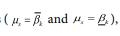 they are calculated as:
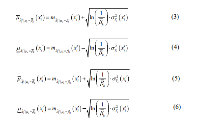
where  represents the center of the fuzzy set
  and
and  and
and  are the upper and lower widths of the fuzzy set
 respectively;
 represents the number of fuzzy rules; represents the number of horizontal slices;
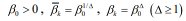 are the upper and lower
where represents a small positive number.
(3) Rule inference layer, The rule inference layer calculates the firing degrees of fuzzy rules based on the membership degrees of input variables. Thej-th fuzzy rule is represented
where  are the upper and lower bounds of the j-th rule consequents, respectively The firing degrees for Eth rule are computed using a
T.norm operation is shown:
are the upper and lower bounds of the j-th rule consequents, respectively The firing degrees for Eth rule are computed using a
T.norm operation is shown:
where  are the upper bound firing degrees of j-th rule at horizontal slices in terms of
are the lower bound firing degrees of j-th rule at horizontal slices in terms of
are the upper bound firing degrees of j-th rule at horizontal slices in terms of
are the lower bound firing degrees of j-th rule at horizontal slices in terms of 
 respectively; and T(*) is the T-norm operator for aggregating input membership degrees.
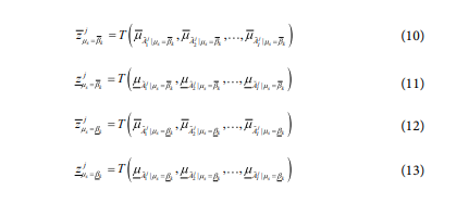
Type-reduction layer: The type-reduction layer combines the firing degrees and rule consequents to compute the consequent values for each horizmtal slice, The calculations are as follows:
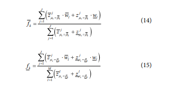
where  are the consequent values at horizontal slices in terms of
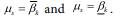
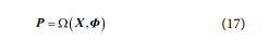
Output layer: The output layer all the consequent values from the type-reduction layer to produce the final system output, Ihe calculation is given by.
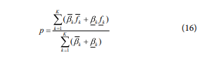
where p is the final system output oflT3FIS with its input
2.2 Broad Learning System (BLS)The BLS is an efficient learning framework designed to achieve fast modeling and training through a shallow and parallel network structure. BLS constructs broad features is [x1,x2],x3...xl]
using feature mapping nodes and enhancement nodes, while optimizing only the weight matrix of the output layen 'Ihis avoids the iterative training process required in conventional deep learning methods. Below, the computational process of BLS is described layer by layer, including the input layer, feature mapping layer, enhancement layer, and output layer.
Input layer: The input layer receives the original data and
forwards it to the feature mapping layer. Assume the value of input data is  where N is the number of samples and D is the dimensionality of the input features. The input layer simply passes the data to the next layer without
performing additional processing.
where N is the number of samples and D is the dimensionality of the input features. The input layer simply passes the data to the next layer without
performing additional processing.
Feature mapping layer: The feature mapping layer performs nonlinear feature transformations on the input data to generate a high-dimensional feature space, as follows,
where  is the output matrix of feature mapping
layer with input X, M is the number of feature mapping
nodes in this layer,
is the output matrix of feature mapping
layer with input X, M is the number of feature mapping
nodes in this layer,  are all parameters of the feature map
layer,
are all parameters of the feature map
layer, and is a nonlinear activation function
Enhancement layer; The enhancement layer further
enriches the feature space by providing additional redundant and nonlinear representations. It takes the feature node
matrix P as input and generates the enhancement node matrix using a randomly initialized weight matrix  using a randomly initialized weight matrix
  using a randomly initialized weight matrix
  and a bias vector
  The computation process of H is defined as
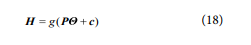
where L is the number of enhancement nodes and g(*) is the nonlinear activation function.
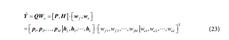
Output layer: The output layer combines the feature node
matrix P and the enhancement node matrix H into a unified feature matrix 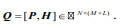 For the target output
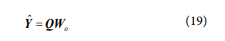
 where c is the output dimension, the predicted output
  is calculated as:
where  represents the weight matrix, which is optimized using ridge regression as follows,
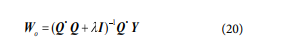
where  the represents the regularization parameter, and I is the identity matrix.
These layers together compute the output of the model to achieve the regression task, The detailed implementation description of each layer is as follows (1) Input layer: The input sample of the input layer can be described

where D is the number of features of the sample. The input X is passed to the interval type-3 fuzzy mapping layer for further processing,
Interval type-3 fuzzy mapping layer: The interval type-3 fuzzy mapping layer consists of M independent IT3FS
units. Each IT3FS receives the input X and computes a mapping output  The outputs of all IT3FS units form the feature matrix in (1)~(16):
This layer provides robust feature mapping under uncertain. ties and serves as the foundation for the subsequent enhancement layer.
Enhancement layer: Ihe enhancement layer expands the
feature space, complementing the outputs of the interval
tvpe-3 fuzz mapping layer. With L enhancement nodes, the
enhancement node output matrix  is
computed using V and c in (18), where
is
computed using V and c in (18), where  Then, the final feature matrix
  is obtained by combining P and H .
Output layer. Utilizing the IT3FS module for feature mapping enables a robust representation of data uncertainty, thereby enhancing the performance of regression modeling tasks [28], The output of IT3FBIS is;
where 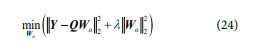 is a weight matrix, connecting the interval
type-3 fuzzy mapping layer, enhancement layer, and output layer.
is a weight matrix, connecting the interval
type-3 fuzzy mapping layer, enhancement layer, and output layer.
To enhance the robustness and generalization performance of the BLS, this article introduces the concept of node-level entropy, which is used to measure the discrete
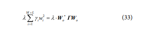
3.2.1 Entropy-Weighted Adaptive RegularizationThe output layer weights of BIS are typically computed layer.
ness of the output distribution of each fuzzy subsystem and enhanced node. This entropy measure is then used to adap- tively adjust the regularization strength for each node within the penalty term.
through classical ridge regression algorithm, with the objective function expressed as:
where  is the regularization coefficient, Y is the true
output of the samples, and the solution for w0 can be derived
from (20),
is the regularization coefficient, Y is the true
output of the samples, and the solution for w0 can be derived
from (20),
The output distributions of fuzzy subsystems within the IT3FS-based mapping layer and enhancement nodes with in the enhancement layer often exhibit significant differences.
To better capture these localized mapping characteristics, information entropy is introduced to quantify the output distribution Of each subsystem or node. This entropy measure is then used to weight the regularization strength, replacing the uniform penalty term with a component-wise weighted form. The modified objective function is given by:
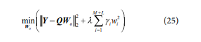
where  represents the regularization weight for the ith
fuzzy subsystem or enhancement node, reflecting the impact
of its distribution entropy on the regularization strength. With
represents the regularization weight for the ith
fuzzy subsystem or enhancement node, reflecting the impact
of its distribution entropy on the regularization strength. With  a larger imposes a stronger penalty on the
corresponding weight, while a smaller value results in a weaker penalty. Ihe specific implementation is as follows:
First, let
a larger imposes a stronger penalty on the
corresponding weight, while a smaller value results in a weaker penalty. Ihe specific implementation is as follows:
First, let  denote the ith column of
matrix ,Q representing the output of the ith fuzzy subsystem or enhancement node for a dataset with N samples.
Define qi, as a random variable representing the distribu-
tion of qi, , whose probability density function (PDF) can
estimated using a Gaussian kernel as:
denote the ith column of
matrix ,Q representing the output of the ith fuzzy subsystem or enhancement node for a dataset with N samples.
Define qi, as a random variable representing the distribu-
tion of qi, , whose probability density function (PDF) can
estimated using a Gaussian kernel as:
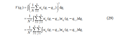
where qin is the nth value of qi, and  is calculated as:
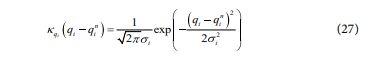
where  the standard deviation of the sample data After obtaining the PDF through kernel density estimation
(KDE), the marginal information potential can be
expressed as:
the standard deviation of the sample data After obtaining the PDF through kernel density estimation
(KDE), the marginal information potential can be
expressed as:

Substituting (26) and (27) into (28) yields:
According to (27),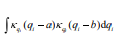 can be computed as:
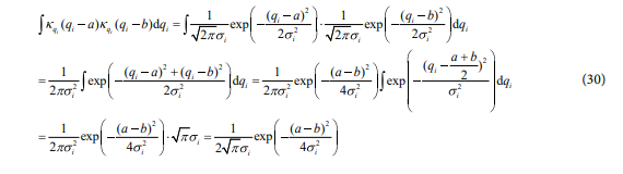
Substituting (30) into (29) gives the discrete form of the marginal information potential qi under the Gaussian kernel as follows:
This calculation requires only N2 kernel function evaluations
to obtain the information potential  Next, for each fuzzy subsystem or enhancement after
calculating its information potential, an exponential mapping function is applied to transform the potential into a regularization weight:

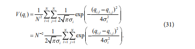
Then, using the diagonal matrix  the
regularized term in (25) can be reformulated as:
the
regularized term in (25) can be reformulated as:
Simplifying the first term in (25) yields:
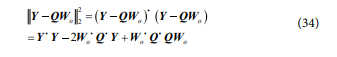
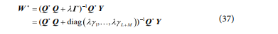
Finally, substitute (34) into (25) , and let be the optimal solution.
By setting the follows:

Let Q' Q = A, We get:
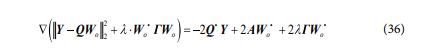
Substituting (35) into (36), the optimal weight of Wo can be calculated as follows:
Notably, by measuring the output distribution entropy of each node and adaptively adjusting the corresponding regularization strength, the proposed approach effectively
3.2.2 Gradient-Based Secondary OptimizationIn the entropy-weight adaptive regularization algorithm described earlier, the output layer weights wo of IT3FBLS can be efficiently computed through entropy-en- hanced ridge regression algorithm. However, the internal parameters of IT3FBIS, including the weight matrix and the bias vector c defined in (18), play a crucial role in network performance but cannot be directly solved using the modified ridge regression algorithm.
If these internal parameters remain initialized through random search or fixed settings, the model's potential cannot be fully exploited. To address this, a gradient descent secondary optimization strategy is introduced, enabling collaborative optimization between output weights and internal parameters during each iteration. This approach enhances both approximation accuracy and convergence speed.
The specific implementation steps for the kth suppresses the influence of abnormal or unstable nodes, thereby improving the generalization performance of the IT3FBLS model.
iteration are as follows:
First, given the training data X and Y , and the current weight matrix p(K) and c(K) the outputs of the fuzzy subsystems O(K) and enhancement nodes H(k) can be calculated using (22). As indicated by (18), the values of p(k) depend solely on X, while H(K) is determined by P(K) , O(k), and C(K)
Second, using KDE as defined in the marginal
information potential for each is estimated. and the
corresponding weighting coefficients  are
derived via (32), These coefficients are then used to
construct the weighted diagonal matrix r(k). The output
layer weights Wo (k) for the current iteration are computed directly via (37).
are
derived via (32), These coefficients are then used to
construct the weighted diagonal matrix r(k). The output
layer weights Wo (k) for the current iteration are computed directly via (37).
Next, for internal parameters 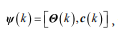 which
cannot be updated through entropy-weighted ridge regression algorithm, GD is applied as follows:
which
cannot be updated through entropy-weighted ridge regression algorithm, GD is applied as follows:

where n>0 is the learning rate, and the specific calculation process follows the [13].
Then, once  are updated, the distribution characteristics of the fuzzy subsystems and
enhancement nodes change accordingly. Therefore, the marginal
information potential and weighting coefficients are recalculated,
leading to an updated weighted diagonal matrix (K + 1) Wo (K+1) The are then updated via (37)
and
are updated, the distribution characteristics of the fuzzy subsystems and
enhancement nodes change accordingly. Therefore, the marginal
information potential and weighting coefficients are recalculated,
leading to an updated weighted diagonal matrix (K + 1) Wo (K+1) The are then updated via (37)
and  are then updated via (38).
Finally, the above steps are repeated until the maximum number of iterations is reached or the convergence criterion is satisfied, thereby completing the gradient-based secondary optimization process for IT3FBLS parameters.
It is worth noting that, under traditional supervised learning frameworks, each update of internal parameters typically necessitates a complete forward pass through the entire network, followed by backpropagation to compute gradients—a process that demands substantial computational resources. In contrast, the proposed parameter learning framework employs an efficient hybrid approach: the output layer weights are computed via a closed-form ridge regression solution, while the internal parameters are locally adjusted using gradient descent. Information potential and the weighted diagonal matrix are recalculated only when necessary. By handling parameter updates in each iteration, the approach leverages the computational efficiency Of ridge regression algorithm alongside the flexibility of gradient descent, allowing the model to rapidly approach an optimal solution.
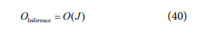
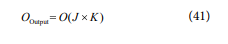
3.3 Computational Complexity analysisIhe compSZutational complexity of the IT3FBLS model is determined by the three main components of its
3.3.1 Complexity of Interval Type-3 Fuzzy Mapping LayerThe interval type-3 fuzzy mapping layer contains architecture: the interval type-3 fuzzy mapping layer, the enhancement layer, and the output layer. The detailed complexity of each component is analyzed in details as follows
independent IT3FS. Each IT3FS computes its output through several stages.
Membership function computation layer computes the membership functions of all input features over j fuzzy rules and k horizontal slices. The complexity is as follows:

For industrial control tasks, N=1.
Rule inference layer: Inference over j rules has a complexity as follows:
Type-reduction layer and output layer: The type-reduction process with the final output computation calculates aggregated outputs over j rules and k slices, with a complexity as follows:
The total complexity of a single IT3FS is:

With M IT3FS units in the interval type-3 fuzzy mapping layer, the total complexity becomes:

The enhancement node layer computes additional feature transformations through L enhancement nodes:
Matrix multiplication: Combining the outputs of the mapping layer with requires:

Activation function: Applying the activation function to L enhancement nodes results in:

The total complexity of the enhancement node layer is as follows:

The output layer computes the output i based on Q . The complexity of the matrix-vector multiplication with Wo is:

Therefore, the total computational complexity of IT3FBIS is the sum of the three components as follows:

In summary, the parameter choices for M , J , K , and L must balance computational complexity and system performance. Among these factors, M is the primary determinant of complexity, and its adjustment has the most significant impact on computational cost. It should be selected within a reasonable range. "Ihe values of K and J primarily affect the complexity of the mapping layer and have a greater influence on real-time performance. These parameters can be reduced when modeling performance demands are low. Ihe growth L of has the least effect on real-time performance and can increased to enhance the model's adaptability and generalization capabilities.
Remark: In the proposed gradient quadratic optimization algorithm, since the most computationally interval type-3 fuzzy mapping layer does not require repeated forward computation, redundant calculations are minimized. Ihis not only reduces computational costs but also ensures the scalability of the prcpsed model for large-scale and real-time applications.
3.4 Algorithm PseudocodeThe pseudocode of the proposed IT3FBIS model is as follows:
Experiments and Discussion
In this section, a systematic study is conducted to evaluate the effectiveness of the proposed fuzzy broad learn. ing system and its associated learning algorithms.
4.1 Modeling Datasets and Evaluation Indicators DescriptionTo ensure a rigorous and comprehensive evalua- tion, three categories of datasets are designed: (1) Benchmark dataset. This dataset employs three represen- tative publicly available datasets for data-driven regression modeling. These datasets include one medium -dimensional and two low-dimensional datasets sourced from the University of California, Irvine (UCI) Machine Learning Repository [291. Ihe aim is to evaluate the proposed algorithm's modeling capability across different data dimem sionalities and complexities. (2) Uncertain function dataset. This experiment investigates the robustness and generalization ability of the proposed algorithm in handling dynamic nonlinearity and high -un- certainty environments. Two classical chaotic systems, the Mackey—Glass time series 1301 and the Rossler attractor [31], are used to test the model's effectiveness in capturing uncertainty-driven behaviors. (3) Complex industrial process dataset. To examine the practical applicability and feasibility of the proposed approach in real-world industrial settings, this experiment applies the algorithm to data-driven modeling tasks in industrial processes. Specifically, it focuses on furnace temB-rature modeling in MSWI [32] and process in the Tennessee Eastman (TE) chemical process 1331. All process data are collected in real time from actual industrial production environments, ensuring a realistic assessment of the algorithm's industrial applicability.
For these datasets, an equal-interval selection strategy is employed, and all datasets are standardized and divided into three subsets: training, validation, and testing. The details Of this partition are presented in Table 1.
To evaluate model performance, three commonly used regression indicators are adopted: root mean square error (RMSE), mean absolute error (MAE), and R2. To ensure a fair evaluation of the simulation results, all experiments are repeated 20 times, and the mean, variance, and optimal values of the evaluation metrics are recorded.
4.2 Hyperparameter Setting DescriptionFurthermore, to validate the effectiveness of the proposed parameter learning algorithm, a comparison is made between IT3FBLS employing traditional ridge regression algorithm (denoted as IT3FBLS-1) and IT3FBLS utilizing entropy-weighted adaptive regularization (denoted as IT3FBLS-2). The hyperparameters of IT3FBLS include the number of fuzzy rules J, number of horizontal slices K, of fuzzy subsystems M, numtber of enhancement nodes L, learning rate , and regularization coefficient A These hyperparameters are determined through a grid search approach, following these steps: First, identify the hyperparameters that require tuning and define a candidate value range for each. Next, enumerate all possible hyperpa- rameter combinations and train the model for each config- uratiom Finally, compare the evaluation results across all configurations and select the combination that yields the best average performance as the final hyperparameter setting. For fairness, the hyperparameter configurations Of other benchmark models in comparison experiments are aligned with those of IT3FBLS as closely as possible. The specific hyperparameter settings used in the experiments are detailed in Table 2.
To comprehensively assess its performance, comparative experiments are performed against the original BLS [23] , classical regression models including FNN [34] and FBLS 35], as well as advanced regression algorithms integrating fuzzy systems and broad learning, including IT2FNN [36] and IT2FBLS [37].
4.3 Results and Discussion 4.3.1 Benchmark datasetThe prediction results and comparison results of the testing set are shown in Fig, 2 and Table 3, In Table 3, the bolded values indicate the two meth- ods for each dataset across different evaluation metrics.
Figure 2 and Table 3 shows that:
1) Comparison with the BLS: On the Housing IT3F. BLS reduces RMSE by approximately 23.6% compared to the original BLS. Ihe MAE decreases, while the R2 improves. These results demonstrate the advantages of IT3FBIS in capturing the complex nonlinear relationships and uncer- tainties present in housing price data.
2) with FNN and IT2FNN: IT3FBIS consis. tently outperforms both FNN and IT2FNN- On the Housing dataset, IT3FBLS achieves a lower RMSE than both FNN and IT2FNN, with corresponding improvements in MAE and RX This suggests that leveraging a higher-order Type-3 fuzzy logic allows for more accurate representation of uncertainty, leading to enhanced predictive performance. Similarly, on the CCS and Abalone datasets, IT3FBIS maintains a lower RMSE and MAE while achieving higher R2. Specifically, rmance improvements over FNN and IT2FNN range from in RMSE and MAE, while R2 increases by 2—6%, further demonstrating the effectiveness of Type-3
4.3.2 Uncertain Function datasetFor uncertain function modeling, the system fuzzy structures in handling complex data.
3) Cnmpared to FBIS and IT2FBLS: IT3FBIS ranks among the best-performing methods across all evaluation metrics, On the Abalone dataset, while FBIS and IT2FBLS achieve strong results, IT3FBIS further reduces RMSE and improves RX IT3FBLS emerges as one of the top two meth- ods in both RMSE and R2, indicating that the entro- py.adaptive regularization and gradient.based secondary optimization mechanisms significantly enhance predictive accuracy and generalization ability.
4) Ablation study Analysis: IT3FBIS-1, which omits the proposed parameter learning algorithm, exhibits a decline in R2, IT3FBIS2, which retains entropy-weighted regular. ization but removes GD-based secondary optimization, shows a similar performance degradation trend. These findings highlight the importance of each hyperparameter module working collaboratively within IT3FBIS. The complete model effectively captures data uncertainty and complexity, leading to consistently lower errors and higher goodness-of-fit across multiple datasets.
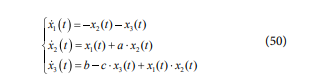
4.3.2 Uncertain Function datasetFor uncertain function modeling, the system dynamics are based on the Mackey-Glass equation and the Rössler attractor equation. The Mackey-Glass equation is formulated as:
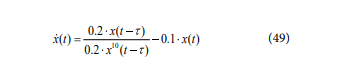
where x(t) is the system state, x(0)=1.1, and t = 20 represents system delay time. The output variable is
 , while the input variables consist of delayed states from multiple
past time steps, including x(t-1), x(t-2), x(t-6), and x(t-12) This equation characterizes the complex nonlinear relation
ship between the current state x(t) and historical states
, while the input variables consist of delayed states from multiple
past time steps, including x(t-1), x(t-2), x(t-6), and x(t-12) This equation characterizes the complex nonlinear relation
ship between the current state x(t) and historical states
 , where higher-order nonlinear terms induce
various uncertain dynamic behaviors such as periodic
solutions and chaotic solutions.
, where higher-order nonlinear terms induce
various uncertain dynamic behaviors such as periodic
solutions and chaotic solutions.
Ihe Rossler system is defined by the following system of equations:
where a = 0- l.b = 0.2.c = 5.7, and the initial condition are
x1(0), x2(0),x3(0)=1,1,1. The output variable  This model exhibits characteristic chaotic dynamics, where
system states are highly dependent on historical states and
exhibit strong nonlinear interactions. Due to the presence of
This model exhibits characteristic chaotic dynamics, where
system states are highly dependent on historical states and
exhibit strong nonlinear interactions. Due to the presence of
nonlinear terms and coupling effects, even minor perturba- lions in initial conditions can lead to significant trajectory divergence, introducing uncertainty into data-driven modeling. The prediction results and comparison results of the testing set are shown in Fig. 3 and Table 4.
Figure 3 and Table 4 show that:
- Comparison with BLS: *Ihe BLS, due to its lack of a fuzzy mechanism, has limited nonlinear modeling capability, resulting in higher prediction errors. In contrast, the IT3F. BLS, which integrates a T3FS, demonstrates significant performance improvements in uncertain function the average RMSE of IT3FBLS is reduced by approximately 95% compared to BLS, with the MAE decreased by 54%. Additionally, R2 significantly increased from 0.25 for BIS to over 0.997 for IT3FBLS. In the Rössler system modeling task, the average RMSE and MAE of IT3FBIS are reduced by 59.46% and 17.14%, respectively, With R2 improving by 0.78, Ihis improvement mainly stems from the effective represen- tation of input-output uncertainties by the third.order fuzzy sets. By deeply integrating the fuzzy feature layer with the BLS broad learning architecture, IT3FBLS achieves more precise mathematical modeling of complex nonlinear relationshi
- Comparison with FNN: IT3FBLS exhibits significant advantages on the Mackey-Glass dataset: the RMSE and MAE are reduced by 41% and 44%, respectively, while increases from 0.9913 to 0.9972. Compared to IT2FNN, the reduction in RMSE and MAE reaches 69%. Notably, in Rössler system modeling, even though FNN has achieved high precision (R2 > 0.99), IT3FBIS still demonstrates stron- ger adaptability. Cmnpared to IT2FNN, its RMSE and MAE are reduced by and 92.8%, respectively. Overall, IT3F. BLS outperforms FNN in most cases, especially in the Mack- eyeGlass task, showcasing the superiority of higher-order fuzzy modeling in handling complex dynamic systems. This indicates that the T3FS, when integrated with BIS, can fit complex mapping relationships more accurately than TIES and T2FS represented by FNN and IT2FNN. The introduction of third -order fuzziness enhances the model's ability to represent uncertainty, leading to significantly better performance on datasets than neural networks using only T2FS.
- Comparison with IT2FNN: IT3FBIS combines the efficient training mechanism of broad learning with the strong uncertainty representation capability of the T3FS. This not only overcomes the limitations of T IFS in modeL ing capability but also addresses the shortcomings of T2FS in handling higher-level uncertainty, The third-order fuzzi• ness, by introducing a degree of membership to the mem- bership degree, effectively describes the credibility range of fuzzy rules, allowing the model to maintain high precision when facing complex noise or unmodeled dynamics. Ihe introduction of BIS provides the ability to quickly expand feature spaces and efficiently solve linear equations, signifi- cantly improving the training efficiency while maintaining high accuracy.
- Cnmparison to FBIS and IT2FBIS: In the Mackey-Glass system, the average RMSE of IT3FBLS is slightly higher than that of FBIS, but its optimal RMSE is close to FBIS, and the optimal value is slightly better than FBIS. While FBIS outperforms IT3FBIS in terms of average perfor- mance, their variances are similar, indicating that models exhibit comparable stability. However, IT3FBLS demonstrates generalization ability in more complex scenarios, In the Rössler system, IT3FBIS reduces the average RMSE by 64.15% and the MAE by 84.55% compared to IT2FBIS, with the optimal RZ value approach- ing the theoretical limit- Given that IT3FBIS introduces a more complex third-order fuzzy uncertainty approach, its advantages are expected to even more pronounced in environments with noise or r uncer- tainty. Therefore, IT3FBLS can be considered to have achieved levels comparable to the most advanced methods, While offering enhanced generalization ability. By more effectively modeling uncertainty, IT3FBLS retains the advantages of ensemble learning and significantly improves predictive accuracy. It combines the ensemble learning characteristics of FBIS with the powerful represen- tational capabilities of T3FS, thus outperforming earlier IT2FBIS Overall, the key improvement oflT3FBIS over existing models lies in its handling of third-order fuzzy uncertainty. FBIS, which uses first-order fuzzy sets, achieves high accuracy but does not explicitly account for the uncertainty in membership degrees, IT2F. BIS introduces uncertainty for degree intervals but may increase model complexity and optimization difficulty. In contrast, IT3FBLS further refines the credibility of the memlkrship function itself through third-order fuzzy sets, offering a more granular uncertainty representation. As a result, IT3FBIS has a potential advan- tage in tasks where generalization ability and noise robust. ness are critical.
- 4) Ablation experiment analysis: In IT3FBIS 1, its perfor- mance significantly declines. In the Mackey-Glass system, the average RMSE of IT3FBIS-1 increases approximately 6S times compared to the full model, with R2 decreasing by about 11%. In the Rössler system, the impact is even more pronounced, with RMSE increasing by more than 750% and RZ dropping nearly 14%. These results clearly indicate that removing the entropy-based parameter learning algorithm leads to a dramatic increase in error and a severe degradation in the model's ability to fit complex relation. ships. In IT3FBLS.2, Experimental results show that in the Mackey-Glass system, the RMSE of IT3FBIS2 is slightly higher than the full model, while in the Rössler system, the average MAE of IT3FBLS-2 increases by 44.7%. "lhis demonstrates that the gradient-based second-order optimization algorithm plays a significant role in suppress. ameter oscillations and im rovin model stability
In this article, the modeling of two complex indus. trial processes, the MSWI process and the TE process, is explored. The description of the MSWI and TE chemical processes and their flow chart are given out as follows.
The MSWI process consists of six stages: solid waste storage and transportation, solid waste combustion, waste heat recovery, steam generation, flue gas treatment, and flue gas emission. Among these, the stability and etficiency of the solid waste combustion stage are directly linked to the overall stable operation of the plant and pollutant emissions 138]. Its process structure is shown in the Figure -4.
The FT is crucial for the combustion efficiency and stability of this stage, necessitating precise control. There are significant differences in the characteristics of MSW between developing countries, such as China, and developed coun- tries, such as those in Europe and America. These differences Often lead to the use Of manual operation modes in many developing countries. In the manual mode, domain experts typically rely on their human brain models to predict the trends of key controlled variables, and then determine the output values of manipulated variables
Tennessee Eastman (TE) process is a complex chemical process with strong variable coupling and nonlin- earity [ The TE process was developed by Eastman Chem. ical Company in the United States to provide a realistic industrial process for evaluating fault detection and variable prediction methods, Its process structure is shown in the Figure 5.
As can be seen in Fig. Gl, the TE prcxess contains eight constituent variables: A, B, C, D, E, F, G, and H. Of these, A, C, D, and E are reactants, B is an inert, G and H are the main products generated by the reactor, and F is a by-product. The dataset selected for this article has a sampling interval of 3mins and contains a total of seven feature variables, namely. A feed (stream l), D feed (stream 2), E feed (stream 3), total feed (stream 4), recycle flow (stream 8) and E component (stream 11) [40].
In the MSWI process, the furnace temperature is a critical variable influencing combustion efficiency, pollutant emissions, and system stability. However, due to the complex composition of waste, uneven combustion charac- teristics, and external environmental disturbances, the furnace temperature exhibits significant nonlinearity,
time-varying behavior, and uncertainty. Therefore, accurately modeling furnace temperature not only aids in optimizing incineration control and improving energy recovery efficiency but also contributes to the effective reduction of pollutants such as dioxins (DXN) and nitro- gen oxides (NOx).
In the TE process, a typical industrial chemical process, involves a reactor where temperature is a key variable determining the reaction rate and product quality. As the system includes complex heat exchange and reaction dynamics, its dynamic Ikhavior also presents significant nonlinearity and uncertainty, 'Ihe sources of uncertainty, sampling intervals, and input/output variables for both the MSWI and TE are summarized in Table 5.
As can be seen in Fig. Gl, the TE prcxess contains eight constituent variables: A, B, C, D, E, F, G, and H. Of these, A, C, D, and E are reactants, B is an inert, G and H are the main products generated by the reactor, and F is a by-product. The dataset selected for this article has a sampling interval of 3mins and contains a total of seven feature variables, namely: A feed (stream l), D feed (stream 2), E feed (stream 3), total feed (stream 4), recycle flow (stream 8) and E component (stream 11) [40].
In the MSWI process, the furnace temperature is a critical variable influencing combustion efficiency, pollutant emissions, and system stability. However, due to the complex composition of waste, uneven combustion characteristics, and external environmental disturbances, the furnace temperature exhibits significant nonlinearity,time-varying behavior, and uncertainty, lherefore. accurately modeling furnace temperature not only aids in optimizing incineration control and improving energy recovery efficiency but also contributes to the effective reduction of pollutants such as dioxins (DXN) and nitrogen oxides (NOx).
In the TE process, a typical industrial chemical process, involves a reactor where temperature is a key variable determining the reaction rate and product quality, As the system includes complex heat exchange and reaction dynamics, its dynamic behavior also presents significant nonlinearity and uncertainty. lhe sources of uncertainty, sampling intervals, and input/output variables for both the MSWI and TE processes are summarized in Table 5.
Figure 6 and Table 6 show that:- Comparison with the BLS: In the MSWI process, the standard BIS performs poorly on the MSWI furnace temperature modeling. Its mean RMSE far higher than IT3F. BLS. This represents a 78.6% reduction in RMSE With IT 3B BLS Likewise, MAE drops about 53.8% lower, BLS's RZ is essentially zero, indicating almost no predictive power, whereas IT3FBLS Exxysts to 0.7455 on average. In fact, the best run of IT3FBLS reaches an R2 of 0.7634, whereas BIS never exceeds 0.08. This huge gain highlights that IT3FBLS can capture the furnace's complex dynamics and uncertain. ties that BLS misses. In more challenging TE process modeling, BLS proves ineffective in tracking system dynamics, while IT3FBIS demonstrates a clear advantage, Unlike BLS, IT3FBIS maintains lower RMSE and a positive R2, showcasing superior modeling capabilities. Quantitative results reveal that IT3FBIS reduces RMSE by over 98% compared to BLS, successfully transforming a previously unusable model into a feasible with moderate accuracy. Although the RZ value of 0.1567 indicates that unexplained variability still exists in the TE reactor temperature, IT3FBLS at least provides a usable model, whereas BLS is entirely unsuitable for this task. This result highlights that the nonlinear modeling capability of IT3F. BIS in the TE prcxess makes it more robust and applicable in complex industrial scenarios.
- Comparison with FNN and the IT2FNN: Both the FNN and the IT2FNN better than BLS on the MSWI problem, but they are outperforrned by IT3FBLS. IT3FBLS yields roughly 50% lower RMSE than FNN and 36% lower RMSE than IT2FNN. In terms of R'. IT3FBLS boosts the explained variance by a large margin (about higher than IT2FNN). These results indicate that IT3FBLS's advanced fuzzy Captures the furnace dynamics much more accurately than the simpler or type-2 fuzzy systems. The type-3 fuzzy logic in IT3FBlS provides a more expressive uncertainty representation. leading to better generalization in this complex process. On the TE process, the fuzzy neural approaches FNN and IT2FNN achieve decent accuracy. IT3FBLS•s mean RMSE is slightly higher than IT2FNN by about 4,796, and its RI is a bit lower than IT2FNN's. However, IT3FBLS achieved the highest best-case R2 on TE This suggests that although run-to-run variability affected its average. IT3FBLS has the capacity to learn a SIFior model Of the reactor under the right conditions. 'Ihe slight shortfall in mean performance could be due to the TE process's characteristics- Nonetheless. IT3FBlSs ability to match the fuzzy neural networks on accuracy while providing a richer uncertainty handling framework is an encouraging sign for its robustness. There- fore, compared to classical fuzzy systems, IT 3FBlS benefits from the BLS which Can integrate features in parallel and solve weights efficiently, combined with type-3 fuzzy logic. The type-I FNN lack• uncertainty modeling, and the IT2FNN handles only interval uncertainty in functions. IT3FBlS extends this to a higher-order fuzzy representation, capturing rnore complex and dynamic uncertainty.
- Comparison to FBLS and IT2FBLS: FBLS and IT2FBLS are advanced ensemble models that combine fuzzy logic With BLS. While FBIS uses Type- 1 fuzzy IT2FBLS employs Typea fuzzy In MSWI process, the FBLS and IT2FBIS models Show improved accuracy over basic BLS and fuzzy networks alone. However. IT3FBLS outperforms both, with RMSE is 32% lower than FBIS and lower than IT2FBLS. IT3FBLS's R' higher than FBIS about 51 % and more than triple IT2FBLS. Even the tk•st-case RMSE Of IT3FBLS is better than the FBIS and IT2FBLS. These gains demonstrate that moving from and type-2 fuzzy logic to type-3 fuzzy logic within the broad learning ensem- ble yields a significant accuracy boost. The MSWI process likely involves uncertainties that type-3 fuzzy BLS handles more effectively, explaining the superior performance, In the TE process. the advanced ensemble models all similarly, with small differences. However, IT3FBLS stands out with best RMSE and best - considerably higher than FBIS's best Or IT2FBISs. This indicates that while IT3F- BLS did not consistently dominate in every run. it has the most potential When conditions are right, likely due to its more expressive model. In practical terms. all ensemble fuzzy RI S mexlels handle the TE reactor problem far better than plain BLS. but IT3FBLS provides the Strongest overall capability, under Varying conditions or if further optimized. In the TE process. when nonlinear factors dominate over uncertainty, the BLS framework is already well-equipped to handle the Core complexities. leading to similar performance among all fuzzy logic-based S variants. Nevertheless, IT3FBLS does not compromise prediction accuracy and at least at the level Of the best-case scenario. This suggests that IT3FBLS retains all the advantages Of IT2FBlS while offering greater potential for improvement in handling uncertainty factors.
- 4) Ablation Experiment Analysis: Ihe full IT3FBIS clearly outperforms its ablations on the MSWI task. "Ihe RMSE of IT3FBLS-1 and -2 are higher than full IT3FBLS. In terms of RZ, full IT3FBIS is about 2-4% higher in absolute terms. IT3FBLS reduces MAE by 3.2% compared to IT3FBLS-2 and 6.3% compared to IT3FBLS- and its RMSE is lower than the best Of -1 Or -2. These differences, though not enormous, are consistent: IT3FBLS is better on every metric than either This indicates that each removed in the ablations does play a role in performance. The full model's superiority on the uncertain MSWI problem that the combination of broad learning and fuzzy logic is synerWStiC — removing parts leads to a noticeable drop in On the TE task. the ablation results are more mixed. IT3F- BLS-2 had a slightly lower mean RMSE than full IT3FBLS and a higher RZ on average. IT3FBlS-l Was a bit Worse. However, as IT3FBLS had the best optimal perfor- mance of the three. This suggests that the full IT3FBLS model has higher capacity or flexibility, which sometimes leads to solutions, but might also rnore variability. The higher variance in IT3FBISs results on TE supports this interpretation — the full model is more complex and Can occasionally overfit Or get Stuck in subopon this dataset. Nonetheless, the fact that IT3FBLS -l and -2 don't consistently outperform the full model confirms that the removed components are general- ly beneficial. In a more uncertainty.dominated setting, those Components likely prove For TE it appears the full IT3FBIS is at least as gcxid as the best ablation on average, and it retains a higher ceiling for performance. With further tuning or ensemble averaging. the full model could likely Surpass the ablations outright even in TE Overall. the type-3 fuzzy component and the ensemble broad feature learning are complementary — the former improves
This section presents a sensitivity analysis Of IT3F model flexibility and uncertainty handling, while the latter ensures strong function approximation and generalization. The ablated models, lacking one of these. cannot consistently match the full IT3FBIS in the face Of complex. uncertain industrial data like MSWI process.
BLS, using the MSWI prcxess dataset as an example. Detailed information about the settings is provided in Table 2.
Fig. 7 shows the results as follows:- (l) The regularization coefficient A significantly affects IT3FBLS performance. When A within the range Of [O, 0.3], R2 shows a notable improvement, indicating that moderate regularization effectively mitigates overfitting- However, once exceeds 03, RI drops rapidly, suggesting that exces- Sive regularization leads to underfitting.
- (2) The number of fuzzy rules J significantly enhances R2 within the 15, 20] range, but when the number exceeds 20, R2 stabilizes, indicating diminishing returns in performance With an increasing number Of rules. Furthermore, When exceeds O, it negatively impacts model performance;
- The number of horizontal slices K leads to the most significant improvement in R2 within the [2. 41 range. but beyond 4, R2 decreases slightly due to feature redundancy. The number of enhancement nodes L generally exhibits a positive correlation With model performance; however, When L exceeds further improvements are marginal.
- The learning rate shows a positive correlation with RI in the ranges 0.41 and [0.45.0.651. but When it exceeds 0.7. large Step Sizes in parameter updates may Cause the model to get stuck in local optima, resulting in perfor- m ance degradation.
- The value Of number Of IT3FS units M maintains high model performance only within the [ 10.2001 range. When exceeding 200. both model and computational time significantly degrade.
Therefore, A and J are highly sensitive hyperparameters with the most significant impact on performance. These should be prioritized for optimization, preferably through grid search or heuristic optimization- L and M also significantly influence model performance and are related to the computational complexity Of the model. Therefore, it is recommended to set reasonable ranges based on domain knowledge to avoid unnecessary expansion- K and to the model is lower sensitive, and their values Can dynamically adjusted through heuristic strategies to balance performance and reduce computational costs.
Conclusion
A novel BIS for uncertain data regression, termed IT3FBLS is in this article. TO the limitations of traditional fuzzy systems in high-order uncer- tainty representation and real-time learning efficiency, is integrated With the BLS framework. This integration facilitates a refined characterization of multi-level uncertain- ties while simplifying the complexity of model parameter learning, Additionally, to address overfitting and enhance generalization capabilities in noisy Of nori-stationary environments. an entropy-based weighted adaptive regular- ization and gradient-based quadratic Optimization parame- ter learning Strategy is in IT3FBLS. This approach dynamically quantifies node distribution and feature contribution. thereby improving robustness to noise and uncertainty. A systematic comparison of IT3FBIS with several conventional methods in the context of uncertainty regression modeling is conducted- are
Declaration of Competing Interest
The authors declare that they have no known
Data Availability
The dataset is available upon request from the corresponding Credit Authorship Contribution Statement
performed Oti Of varying scales and dimensions, uncertain functions, and real-world industrial data. The results demonstrate that IT3FBIS achieves superior and stability With a limited Of training samples. More-over, it exhibits lower on hyFrparameters when handling multi-source heterogeneOuS data and high-dimensional noise. showcasing its inherent robustness and adaptability. Notably, IT3FBLS maintains strong Frformance across diverse scenarios. remaining insensitive to changes in data dimension and scale. These findings underscore the method's potential for high-dynamic industrial pr€xesses and other uncertainly-driven applications.
Future research on further reducing the computational overhead of IT3FBIS while enhancing its efficiency and stability in practical industrial applications, such as real-time control and online Additionally, advanced ensemble learning mecha- nisms. parameter learning. and incremental learning methods into the IT3FBLS framework is to essential for addressing challenges Such as distribution drift and multi- task collaboration in dynamic environments.
competing financial interests or personal relationships that could have appeared to influence the work reported in this
Hao Tian: Methodology, Validation, Data Curation, Writing - Original Draft.
- Y. Chen, C. Wang, Y. Zhou, Y. Zuo, Z Yang, H. I-i, and J. Yang. Research on multi-source heterogeneous big data fusion method based on feature level. International Journal of Pattern Recognition and Artificial Intelligence, vol, 38, no, 02 (2024): 2455001.
- W. Shao, C Xiao, J. Wang, D. Zhao, and Z Song. Real-time estimation of quality-related variable for dynamic and non-Gaussian process based on semisuFrvised Bayes. ian HMM. Journal of Process Control, vol. 111 (2022): 59-74.
- W. Yu, C. Y. Wong, R. Chavez, and M. A. Jacobs. Integrating big data analytics into supply chain finance: roles of information prcxessing and data-driven culture. International journal of production economics, vol. 236 (2021): 108135.
- A. M. Khedr, I. Arif, M. El-Bannany, S. M. Alhashmi, and M. Sreedharan. Cryptocurrency price prediction using traditional statistical and machine-learning techniques: A survey. Intelligent Systems in Accounting, Finance and ement, vol. 28, no. 1(2021): 3-34
- I, H. Sarkr, A1-based modeling: techniques, applications and research issues towards automation, intelligent and smart systems. SN computer science, vol. 3, no. 2 (2022): 158.
- C Li, Y. Chen, and Y. Shang. A review of industrial big data for decision making in intelligent manufacturing. Engineering Science and Technology, an International Journal, VOL 29 (2022): 101021.
- J. M. Mendel. Fuzzy logic systems for engineering: a tutorial. Prcxeedings of the IEEE, vol. 83, no. 3 345-377.
- J. Fei, Z Wang, X. Liang. Z Feng, and Y. Xue- Fractional sliding-mode control for microgyroscope based on multilayer recurrent fuzzy neural network. IEEE transactions on fuzzy systems, vol. 30, no. 6 (2021): 1712-1721.
- H, Ding, J, Qiao, W. Huang, and T. Yue Cooperative event-triggered fuzzy-neural multivariable control with multitask learning for municipal solid waste incineration process. IEEE Transactions on Industrial Informatics, VOL 20, no. 1 (2023): 765-774.
- J. Y. Ho, J. Ooi, Y. K- Wan, and V. Andiappan, Synthesis of wastewater treatment process (WWTP) and supplier selection via Fuzzy Analytic Hierarchy Prcxess (FAHP). Journal of Cleaner Production, vole 314 (2021): 128104.
- N. N. Karnik. J. M. Mendel. and Q. Liang. Type-2 fuzzy logic systems. IEEE transactions on Fuzzy Systems, vole 7,no. 6 (1999):643-658
- Q. Liang, and J. M. Mendel. Interval type-2 fuzzy logic systems: and design. IEEE Transactions on Fuzzy systems. vol. 8, no. 5, (20(X)): 533-550.
- H. Tian, J. Tang, H. Xia, W. Yu, and J. Qiao. Bayesian interval type-2 fuzzy neural network for furnace temperature control. IEEE Transactions on Industrial Informatics, vol. 21, no. 1, (2025):505-514.
- O. Castillo, Towards finding the optimal in designing type-n fuzzy systems for particular classes of problems: A review, AppL Comput. Math.. vol. 17, no. 1. (2018): 3-9.
- Y. Chen and D. Wang, Study on centroid type-reduction of general type-2 fuzzy logic systems with weighted Nie—Tan algorithms, Soft Comput., vol. 22, no. 22, (2018): 7659-7678.
- J. R. Castro, M. A. Sanchez, I. Gonzalez, P. Melin, and O. Castillo, A new method for parameterization of general type-2 fuzzy sets, Fuzzy Inf. Eng., vol. 10, no. 1, (2018): 31-57.
- P. Melin and D. Sånchez, Optimization of type-I, interval type-2 and general typ2 fuzzy inference systems using a hierarchical genetic algorithm for modular granular neural networks, Granular Comput., vol. 4, (2019): 211-936.
- A. Mohammadzadeh, M. H. Sabzalian, and W. Zhang. An interval type-3 fuzzy system and a new online fraction. al.order learning algorithm: theory and practice. IEEE Transactions on Fuzzy Systems, vol. 28, no. 9 (2019): 1940-1950.
- Z Liu , A. Mohammadzadeh, H. Turabieh , M. Mafarja, S, S. Band , A. Mosavi. A new online learned interval type-3 fuzzy control system for solar energy management ems. IEEE Access, vol. 9, (2021): 10498-10508.
- L Amador-Angulo, O J. R. Castro , P. Melin. A new approach for interval type-3 fuzzy control of nonlinear plants. International Journal of Fuzzy Systems, vo. 25, no, 4, (2023): 1624-1642.
- P. Ochoa, O. Castillo, P. Melin, J. R. Castro. Interval type-3 fuzzy differential evolution for parameterization of fuzzy controllers. International Journal of Fuzzy Systems, VOL 25m no. 4, (2023): 1360-1376.
- D. J. Singh, N. K. Verma, and A. Ki Ghosh, Appasaheb Malagaudanavar. An approach towards the design of interval type-3 T–S fuzzy system. IEEE Transactions on Fuzzy Systems, vol. 30, no. 9, (2021): 3880-3893.
- C L P. hen , and Z Liu. Broad learning system: An effective and efficient incremental learning system without the need for deep architecture. IEEE transactions on neural networks and learning systems, vol. 29, no .1, (2017): 10-24.
- X. Gong, T. Zhang, C. L. P Chen, and Z. Liu. Research review for broad learning system: Algorithms, theory, and applications. IEEE Transactions on Cybernetics, vol. 52, no. 9, (2021): 8922-8950.
- S. Feng, and L P. Chem Fuzzy broad learning system: A novel neuro-fuzzy model for regression and classification. IEEE transactions on cybernetics, vol. 50, no. 2, (2018): 414-424.
- Y. Zhou, Q. Zhang, H. Wang, P. Zhou, and T. Chai, EKF-based enhanced performance controller design for nonlinear stochastic systems, IEEE Trans. Autom. Control, vol. 63, no. 4, (2028): 1155–1162.
- L. Yin and L. Guo, Fault isolation for multivariate nonlinear nonGaussian systems using generalized entropy optimization principle, Automatica, vol. 45, no. 11, (2009): 2612–2619.
- H. Tang, P. Dong, and Y. Shi, A construction of robust representations for small data sets using broad learning system, IEEE Trans. Syst., Man, Cybern. Syst., vol. 51, no. 10, (2019): 6074–6084.
- C. L. Blake and C. J. Merz. (1998). UCI Repository of Machine Learning Databases. Dept. Inf. Comput. Sci., Univ. California, Irvine, Irvine, CA, USA. [Online]. Available: http://archive.ics.uci.edu/ml/datasets.html
- G. Leon, and M. Mackey. Mackey-glass equation. Scholarpedia, vol. 5, no. 3, (2010): 6908.
- R. Marat, and J. M. Balthazar. On an optimal control design for Rössler system. Physics Letters A, vol. 333, no. 3-4, (2004): 241-245.
- H. Tian , J. Tang, and T. Wang. Furnace temperature model predictive control based on particle swarm rolling optimization for municipal solid waste incineration. Sustainability, vol. 16, no. 17, (2024): 7670.
- B. Andreas, N. L. Ricker, and M. Jelali. Revision of the Tennessee Eastman process model. IFAC-PapersOnLine, vol. 48, no. 8, (2015): 309-314.
- D. C, Souza, P, Vitor- Fuzzy neural networks and neuro-fuzzy networks: A review the main techniques and applications used in the literature. Applied soft computing, vol. 92. (2020): 106275.
- S. Feng , C. L P. Chen, L Xu, and Z Liu. On the accuracy—complexity tradeoff of fuzzy broad learning system. IEEE Transactions on Fuzzy Systems, vol. 29, no. 10, (2020): 2963-2974.
- Z. Sun, X. Meng, and J. Qiao. An IT2FNN with a Novel Hierarchical Learning Algorithm for Nonlinear System Modeling. In 2023 China Automation Congress(CAC), pp. 2848-2853. IEEE, 2023.
- H. Han, H Liu, J Qiao, and C. L. P. Chen. Type-2 fuzzy broad learning system. IEEE Transactions on Cybernetics, vol. 52, no. 10, (2021): 10352-10363.
- J. Tang, H. Xia, W. Yu, and J. Qiao, Research status and prospects of intelligent optimization control for municipal solid waste incineration process, Acta Anat. Sin., vol. 49, no. 10, (2023): 2019-2059.
- X. Gao, and J. Hou, An improved SVM integrated GS-PCA fault diagnosis approach of Tennessee Eastman process, Neurocomputing, vol. 174, part. B, (2026): 906-911.
- Y. W. Zhang, Y. D. Teng, and Y. Zhang, Complex process quality prediction using modified kernel partial least squares, Chem. Eng. Sci., vol. 65, no. 6, (2010): 2153-2158.
Algorithm 1
Algorithm 1 IT3FBLS modeling algorithm |
|
Input: Training data {X, Y}; Initial model parameters; Regularization parameter; Learning rate; Maximum iteration number |
|
Output: Model prediction output |
|
(1). Initialization |
Compute the outputs of the fuzzy subsystems P and enhancement nodes H // ~ |
Concatenate P and H to construct matrix Q, and calculate the initial model prediction output |
|
(2). Calculate information entropy and regularity coefficient |
For each column of Q , estimate the PDF using KDE and calculate the corresponding information entropy // ~ |
Apply the exponential mapping function to transform the entropy into regularization weights and construct the diagonal matrix |
|
(3). Update |
Update the output layer weights |
(4). Gradient descent for internal parameters: |
Compute the gradient of loss function with respect to |
(5). Gradient-based secondary optimization |
After updating |
Update the output layer weights again using the updated |
|
Repeat Steps 2 through 5 until the maximum number of iterations is reached. |
|
(6). Output results |
After IT3FBLS training is completed, the model prediction output |
Algorithm 1 The pseudocode of the proposed IT3FBLS model is as follows:
FIGURE 1
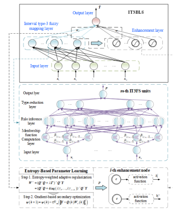
Figure 1: IT3FBLS structure
These layers together compute the output of the model to achieve the regression task. The detailed implementation description of each layer is as follows.
FIGURE 2
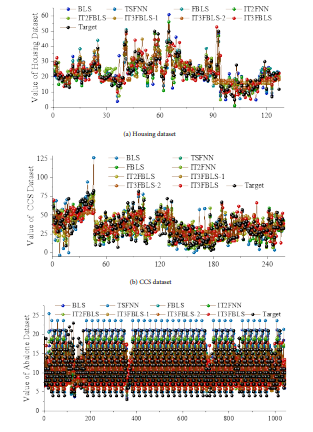
Figure 2: Prediction results of the testing set for the benchmark datase
FIGURE 3
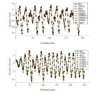
Figure 3: Prediction results of the testing set of uncertain function dataset
FIGURE 4
Figure 4:MSWI process flow diagram
FIGURE 5
Figure 5:Structure diagram of Tennessee Eastman process
FIGURE 6
Figure 6:Prediction results of the testing set of complex industrial process data sets
FIGURE 7
Figure 7:Parameter sensitivity of IT3FBLS
Tables at a glance
Figures at a glance