Physics Informed Neural Network to Understand Multimeter
Received Date: August 11, 2025 Accepted Date: August 22, 2025 Published Date: August 29, 2025
doi:10.17303/jaist.2025.2.204
Citation: Vishal VR Nandigana (2025) Physics Informed Neural Network to Understand Multimeter. J Artif Intel Sost Comp Tech 2:1-9
Abstract
In this paper we develop physics informed neural network model to obtain parameters of the multimeter design. We design the voltage and current of the multimeter. We consider fixed geometry of length 0.5 m. The area is 0.025 m2. The model uses generalized partial differential equation (PDE) that are included in the neural network. Our distributed neural network are trained. We use 10 train sets to calculate the voltage. The train set 1 have input variables [grid location, voltage and concentration]. Each train set have 100 rows. It is due to the grid points. We have 300 numbers in the train 1 file. We have 3000 numbers in our training data of 10 files. The concentration are varied in this fashion [Train 1 = 1000 mM, Train 2 = 1 mM, 2 mM, 5 mM, 10 mM, 20 mM, 50 mM, 100 mM, 200 mM and Train 10 = 500 mM]. The model predicts for 1 test set. The test set have [grid location and new concentration]. We study fixed concentration of 1200 mM. Our results are accurate in multimeter sensor for voltage. Further, we use 10 train sets to calculate the current. The train set 1 have input variables [grid location, current and voltage]. The voltage in the train set are [Train 1 = 1 V, Train 2 = 2 V, 3V , 4V to 10 V]. We predict for test voltage in our multimeter. The test voltage is 11 V. We obtain conservation of current and high accuracy. The multimeter sensor and their parameters includes electrolyte diffusion and concentration are available in our model.
Keywords: Physics Informed; Neural Network; Artificial Intelligence; Machine Learning; Multimeter
Introduction
Neural networks are classes that have array informed to match the result. Machine learning is computer program that is subset of neural network. In order to obtain result the program is used to obtain and learn the train numbers [1]. The advancements of underwater rover from data driven science in sensors are tremendous [2]. The research on sensor to this area of vehicle movement lacks precision in battery, multimeter and their voltage-current measurement. In order to solve the sensor problem the use of computer, data, mathematical model, battery and multimeter components, solvents, chemicals, electrical wiring, digital readings and thin film needs to be known in thorough [3-5]. The train numbers are battery design and multimeter component variables.
Neural network is a computational program that is inspired from the human brain to integrate the machine learning and give a logic to obtain answers when new numbers in the components are given. The component in this study is multimeter. The logic in recent studies in neural network are Rectified Linear Unit (ReLU) program [6]. In machine learning the program learns from the data and provides the weight. The learning data are called Training sets. The neural network used nowadays are artificial neural network (ANN), convolutional neural network (CNN), recurrent neural network (RNN) and Long Short-Term Memory (LSTM). Each of these neural networks have machine learning habit in the program. The neural networks learn the training sets of data and process them to optimize the weight. The least squares method is used to obtain optimal weight. The epoch is a number that specifies the number of iterations used to minimize the error while obtaining the weight [7].
In recent studies the machine learning regression model is used to understand the tensile strength, yield stress and elongation at fraction of steel coils [8]. Here Random Forest Regression is used. The multimeter has steel components. The purpose of multimeter is to understand the continuity of network coming from the input power supply. The load connecting the power supply draws the current. The behavior of the electrons in the wire and load are measured using multimeter. The typical readings of the load and electrical wirings in the multimeter are voltage, resistance and current. Typically we call the load that are predominantly used as motors, fans, pressure sensors, medical devices and advanced sensors. The input power supply are battery, printed circuit board (PCB), switched-mode power supply (SMPS) and electrical plug. The model is necessary to understand the behavior of multimeter.
We use spring, knobs, buttons and their properties are must. The algorithm provides insights on the important features or properties and their relation with other features. Extreme Gradient Boost is used to minimize the error in entry of the data. The extreme gradient boost uses gradient descent algorithm. Support Vector Regression (SVR) is used to ensure the data is continuous. SVR gives the best fitting function for the data. Artificial Neural Networks are used for the training and accurately predict the steel properties. The chemicals are membrane and electrolyte in the multimeter. Now graphene is researched from visual imaging machine learning model [9]. The computational cost of the machine learning model are many orders of magnitude lower than theory. Electrochemical reaction and sensor of multimeter is new area of research that is using machine learning model [10]. Neural network with sensor readings are researched to obtain precision measurements and devices [11,12].
The rest of the paper is as follows. The physics informed from PDE in the neural network are provided in section 2. Section 3 have the architecture of physics informed neural networks. The results and discussion are given in section 4. The conclusions are given in section 5.
Physics Informed From Partial Differential Equation and Distributed Artificial Neural Network Model
Governing Equations
In this section we provide generalized partial differential equation (PDE) for solid-liquid, electrical, instrument noise and physics based noise. The equation for transport has convective, electric component, charge components, physics based noise and box model. Under such conditions the physics of transport phenomena for electrolytes are given by Eq. (1).
Where u is velocity, ρ is the density, v is the volume and Φ is the electric potential. q is the charge. We model the velocity gradient. k is Boltzmann constant, G is conductance, T is temperature and BH is the frequency instrument. AL is the charge carrier of solvent chemicals and fL are the frequency term. I is the current. The current is calculated by integrating the flux (Γ) over the cross-sectional area given in Eq. (2).
Where S is the cross-sectional area of the multimeter, z is the valence, F is Faraday’s constant. The flux of the electrolyte is contributed by the potential gradient given by Eq. (3).
Where D is the diffusion coefficient of electrolyte, R is gas constant and c is the concentration of the electrolyte.
Substituting Eq (3) in Eq (2) and integrating over the cross section area we obtain the current in Eq (4).
We have to define the electric field in our physics.
The electric field E is constant. Lx is the length of the multimeter. The conservation of current is sensor technology. The current is calculated using Eq (6).
We assume no velocity in our model. We consider steady state. We assume no square root noise term. We solve the PDE using finite volume method.
Simulation Details
In our 1D PDE for the voltage study we vary only the concentration. We consider fixed geometry length = 0.5 m. Here area is 0.025 m2. We consider diffusion coefficient D = 2 × 10⁻⁹ m2/s. First we divide the number of length points to 100. The charge carrier is 760C.
The frequency term is 0.28 mHz. This corresponds to time 1 hour. The current from the charge carrier and frequency term is 0.21 A.
In our 1D PDE for the current study we vary only the voltage. The voltage used are from 1 V to 10 V. The electric field is obtained. We consider fixed geometry length = 0.5 m. We consider fixed concentration of 1000 mM.
Architecture of Physics Informed Neural Networks Voltage Study
Here, we develop Physics informed neural networks (PINNs) having two modules to study multimeter. The train module and test module. The train module receives the variables from partial differential equations. The details of the train module are given here.
Step 1: Provide grid locations, variables in the partial differential equation that includes the concentration and voltage. The number of grid points are 100 the grid points are provided in rows. For each row the variables [voltage and concentration] are given. Here, we do not vary the geometry. We study 1D PDE. Here the length of the multimeter is 0.5 m. The concentration parameter for each training are given. [concentration = 1 mM, 2 mM, 5 mM, 10 mM, 20 mM, 50 mM, 100 mM, 200 mM, 500 mM, 1000 mM]. The 1D PDE is used to obtain voltage for each concentration. We use 10 training sets. Table 1 shows the parameters of some grid locations, voltage and concentration for training 1. The rows are the layers in our model.
Step 2: The least squares method are used to optimize the train data and obtain the weight in the neural network. The Adam optimizer in python are used. The weight parameters are optimized. They are obtained from fitting methods on the provided 10 training set of data. Hence it is a network. We use minimal training set in this study. This reduces the computational cost.
Step 3: We provide the test data. We study one test dataset. We study for concentration 1200 mM. The same grid locations are used in the test study. Here the optimized weights from the training data are used. Also, we use Rectified Linear Unit (ReLU) neural network with the training data. We use sequential method in the neural network in python. We use prompt shell. We use predict function in python with verbose =1 to compile the network model.
Current Study
Here, we develop Physics informed neural networks having two modules to study current in the multimeter. The train module and test module. The train module receives the variables from partial differential equations. The details of the train module are given here.
Step 1: Provide grid locations, variables in the partial differential equation that includes the current and voltage. The number of grid points are 100. The grid points are provided in rows. For each row the variables [current and voltage] are given. Here, we do not vary the geometry. We study 1D PDE. Here the length of the multimeter is 0.5 m. The voltage parameter for each training are given. [Voltage = 1V to 10 V]. The 1D PDE is used to obtain current for each voltage. We use 10 training sets. Table 2 shows the parameters of some grid locations, current and voltage for training 1. The rows are the layers in our model.
Step 2: The least squares method are used to optimize the train data and obtain the weight in the neural network. The Adam optimizer in python are used. The weight parameters are optimized. They are obtained from fitting methods on the provided 10 training set of data. Hence it is a network. We use minimal training set in this study. This reduces the computational cost.
Step 3: We provide the test data. We study one test dataset. We study for voltage 11 V. The same grid locations are used in the test study. Here the optimized weights from the training data are used. Also, we use Rectified Linear Unit (ReLU) neural network with the training data. We use sequential method in the neural network in python. We use prompt shell. We use predict function in python with verbose =1 to compile the network model.
Results and Discussion Voltage Design
Figure 1 shows the voltage variation with the grid points for the multimeter. This is our train set 1. The train set having [grid location, voltage and concentration]. The plot is for 1000 mM concentration of the electrolyte chemical in the sensor.
The training set we call Train 1 having 100 rows. We create 10 Training sets having 100 rows. We study for concentration in the train set given as [1000 mM, 1 mM 2 mM, 5 mM, 10 mM, 20 mM, 50 mM, 100 mM, 200 mM and 500 mM]. We test for 1 set only. The concentration in the test set is 1200 mM. The grid locations are same. The least squares method is used to optimize the train data and obtain the weight in the neural network. We use ReLU neural network. We use sequential method with neural network in python. We use prompt shell.
Figure 2 shows the magnitude of voltage is reasonable in our physics informed model. The direction of the voltage relevant to sensor first principle of electric field for the first time. The change in the reading are available in the physics. The accuracy of voltage are permissible in the multimeter design.
Current Model
We use training set 1 given [grid location, current and voltage]. The voltage is 1 V. The voltage is varied from 1 V to 10 V for our training set 1 to training set 10. We save each training set as 1 file. This leads to training files of 10. Using our model we predict the current. The test set are [same grid location and new voltage]. The new voltage is 11 V. Figure 3 shows the comparison of predict and PDE current along the length grid location. The current is conserved. The number of points are 100. The epoch is 200. The accuracy is good and physics of model with diffusion admissible are available. The simulation takes few seconds. The current in conservation from physics are needed. The neural network with current conservation ensures material fluid electrolyte working capability in design and manufacturing.
The physics of valence needs to be included in the physics informed neural network for the multimeter model. The prediction for many test cases should be provided. The prediction should be provided for accurate answers to grid locations. The accuracy of the model with no dependence on the column to predict the voltage and current should be provided. The sensitivity of the model presented here has to be studied for different load devices.
Conclusions
To conclude we model using our physics informed PDE that is included in our neural network to study multimeter. We obtain that physics and field calculations are available in the voltage. The current is conserved in our model. The accuracy is good. The parameters of solvent, chemicals, electrolyte, geometry and components are available in our model. The model can find applications in multimeter and sensors.
Acknowledgments
There is no funding for this work.
Author Contributions
Nandigana V. R. Vishal: Conceptualization, Data curation, Formal analysis, investigation, methodology, re-sources, software, supervision, validation, visuali-zation, writing – original draft, writing – review and editing.
Data Availability Statement
The data are available upon request.
Conflicts of Interest
The author declare no conflict of interest.
- M Raissi, P Paris, EK George (2019) Physics informed neural networks: A deep learning framework for solving forward and inverse problems involving nonlinear partial differential equations, Journal of Computational Physics. 378: 686-707.
- P Norvig, SJ Russes (2009) Artificial Intelligence: A Modern Approach, Prentice Hall.
- A Ali, RA Tufa, F Macedonio, E Curcio, E Drioli (2018) Membrane technology in renewable- energy-driven desalination. Renew. Sustain. Energy Rev. 81: 1–21.
- https://www.sigmaaldrich.com/IN/en/product/mm/101255
- K Gerstandt, KV Peinemann, SE Skilhagen, T Thorsen, T Holt (2008) Membrane processes in energy supply for an osmotic power plant, Desalination 2024: 64–70.
- I Goodfellow, Y Bengio, A Courville (2016) Deep Learning, MIT Press.
- N Lux, C Mandal, J Decker, J Luboeinski, J Drewljau, et al. (2024) HPC AI benchmarks - A comparative overview of highperformance computing hardware and AI benchmarks across domains, Journal of Artificial Intelligence & Robotics, 1: 1-14.
- G Millner, M Mucke, L Romaner, D Scheiber (2023) Machine learning mechanical properties of steel sheets from an industrial production route, Materialia. 30: 101810.
- Rowe P, Csanyi G, Alfe D, Michaelides A, (2018) Development of a machine learning potential for graphene, Phys. Rev. B. 97: 054303.
- Z Zheng, F Florit, B Jin, H Wu, SC Li, et al. (2025) Integrating Machine Learning and Large Language Models to Advance Exploration of Electrochemical Reactions, Angewandte Chemie. 64: e202418074.
- J Payette, F Vaussenat, S Cloutier (2023) Deep learning framework for sensor array precision and accuracy enhancement, Scientific Reports. 13: 11237.
- Z Ballard, C Brown, AM Madni, A Ozcan (2021) Machine learning and computation-enabled intelligent sensor design, Nature Machine Intelligence. 3: 556–65.
FIGURE 1
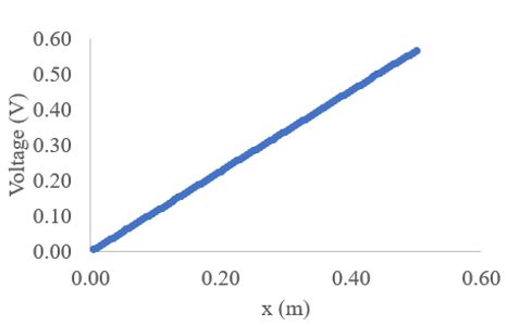
Figure 1: The voltage variation along the grid points. Here concentration is 1000 mM. This is data of training set 1.
FIGURE 2
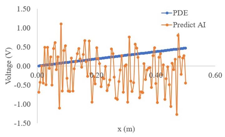
Figure 2: shows the comparison of the predict and PDE voltage variation with the grid points for the multimeter. The test concentration is 1200 mM. Here we use epoch = 200.
FIGURE 3
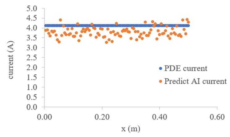
Figure 3: shows the comparison of the predict and PDE current variation with the grid points for the multimeter. The test voltage is 11 V. Here we use epoch = 200.
Tables at a glance
Figures at a glance