Investigation of the Distance Time of Polystyrene Under the Application of DC Motor Having Rollers
Received Date: January 13, 2026 Accepted Date: February 09, 2026 Published Date: February 12, 2026
doi:10.17303/jaist.2026.3.101
Citation: Nandigana V R Vishal (2026) Investigation of the Distance Time of Polystyrene Under the Application of DC Motor Having Rollers. J Artif Intel Sost Comp Tech 3: 1-20
Abstratct
In this paper we study the distance traveled with time for light weight polystyrene polymer material. The polystyrene is transported using non-contact method. We have switched mode power supply (SMPS) that have 12 V DC voltage. It has electrical plug connected to 220 V AC supply. The switched mode power supply have AC to DC converter. We have controller in the device that regulates the voltage from 0 V to 12 V. However, we study the transport upto 8 V. The controller is connected to DC motor having rollers. The maximum voltage of DC voltage are 12 V and current is 1.2 A, respectively. The controller is used to control the voltage and current of the DC motor having rollers only. The polystyrene is next to the DC motor. The length of the polystyrene is 2 cm, width is 2 cm and thickness is 0.082 mm. The volume of the polystyrene are 3.28 × 10⁻⁸ m3. We use digital precision balance to measure the mass of the polystyrene. The mass is measured value of 34 milligram. We obtain no transport upto 4 V. The distance traveled by the polystyrene are 0.2 cm for 5 V at time 7 s. For 6 V, 1 cm at 27 s, 7 V it is 2 cm at 16 s and 8 V the distance is 3 cm at 5 s. The polystyrene stops after the said travel. The wind energy from DC motor having rollers can push multiple polystyrenes. Here, we study single polymer. The wind energy pushing the polystyrene needs further study with regard to air element contact on the material for the push and final stop. We develop data driven neural network to match the distance for given time. The accuracy of the models are good. The computer time are 35 s for training and 0.09 s for predict. We use limited 3 or 4 training data set. We use 1 test set to predict. The simulations are run in a computer. Our work can find applications in low power devices, portable, material handling manufacturing, sensors, embossing, energy and packaging.
Keywords: DC Motor; Rollers; Polymers; Molecules; Distance; Velocity; Acceleration
Introduction
The dynamics of transport have evolved from the structure. The dynamical equation to model the electron flow in the polymers are studied in detail. In polymers the electron mobility is known [1-5]. The molecules, charges and the materials inside the polymer are also studied. The dynamical properties are the distance, velocity and acceleration. The polymers are lightweight materials [6]. The study of mass of polymers are needed. There are recent studies to understand the valence contribution of atoms, electrons and ions from the first principles simulations [7- 13]. The principle dynamics of polymer under the action of force causes external motion. Here, we study polystyrene. Polystyrene like polyethylene oxide also have carbon and oxygen. Along with them small traces of calcium are available [14]. The composition of the elements are obtained from energy dispersive spectroscopy. Polystyrene are thermoplastics. Polystyrene is thermally stable below 200 ◦C. The surface roughness in relation to the chemical elements and size should be the scope for the future. Researchers have studied polystyrene from the ethylene and benzene hybridization fabrication methods [13, 15]. The substrate studies of polystyrene are available [16]. The source, detection and interaction of polystyrene with liquid are studied [17-21].
In the recent years the machine learning (ML) of polymers are studied. The ML methods are used to discover new materials in the polymers [22-26]. The availability of data and experiments for polymers are limited. The study of polymers are taken from the membranes, packaging and 3D printing. ML methods are to provide details of the polymer using Random Forest Regression, Extreme Gradient Boost, and Support Vector Regression (SVR). The clustering of polymers to solid, liquids, understanding the features and properties of polymer are available in the ML literature. The pipeline using ML methods for polymers are well studied. The study of deep learning neural network algorithms for polymers are limited.
Further, there is literature towards metal-ion in polymer matrix. The fundament transport and its mechanism inside the polymers are studied. There are studies to understand the device transport using polymers [27-31]. The architecture of polymer from modeling confirmation is missing in the literature. The compositions in the polymer defines the polymer architecture. Some of the mechanical properties were found in polymers. The structure and morphology change in polymers are less understood. They have implications to change the properties and simulation formula for polymers [32-35]. The use of polymers their ions are towards synthesis of polymers, electrode and voltage devices.
In this paper, we build experiment set up to understand the distance time travel of the polystyrene material under the application of external DC motor having rollers. The DC motor are powered by the switched mode power supply. The controller gives the range of power to study the transport of the polymer. Figure 1 shows the schematic illustration of the distance traveled by the polystyrene. The polystyrene is placed on the white sheet and its transport is examined by external DC motor having rollers. We study non-contact polystyrene transport.
The rest of the paper is outlined as follows. Section 2 discusses the materials and methods. The experiment methodology are given in section 3. The theory for the polymer transport are given in Section 4. The neural networks simulations that include the data driven neural network and physics from theory in the neural network are given in section 5. A detailed discussion is provided in section 6. Finally, conclusions are presented in Section 7.
Materials and Methods
Here, we purchase the polystyrene from Lakshmi electricals and Hardware, India. We use cutter to cut the polystyrene to our size given in the paper. We purchase cutter from Nimibind, India. We study the size of the polystyrene using plastic scale, digital vernier and micrometer. The micrometer measures the thickness of the polystyrene. The micrometer and plastic scale are purchased from Progressive Trade, India. The digital vernier caliper are purchased from Industry buying, India. We purchase OM camera. It has microscopy imaging. The OM camera is purchased from Kesari Scientific Chemicals, India. We measure the mass using Kern mass balance. The mass balance accuracy is 0.01 g. It can measure maximum 1200 grams. The mass balance is purchased from Merck, Germany. The switched mode power supply is purchased from Velonix, India. The controller, DC motor having rollers are purchased from Velonix. India. The acrylic base unit to mount the SMPS, controller and DC motor having rollers are fabricated from IITM facility. The electrical wirings are connected. The multimeter port terminals are provided on the acrylic base unit using fabrication facility at IITM. The electrical wirings are connected to the digital multimeters. The multimeters are purchased from electronics, India. The multimeter measures the voltage of the SMPS, voltage of the controller, voltage and the current of the DC motor having rollers. We use four multimeters. The digital temperature sensor are purchased from Industry buying, India.
Table 1 shows the equipments used in the study. We have switched mode power supply, controller, DC motor, acrylic slab to mount the devices. The multimeter terminals are placed on the acrylic slab. We use four multimeters. The multimeters are used to measure the voltage and current, respectively. The electrical wirings are available. The chart papers are available on the acrylic slab. The book table of the same height as the acrylic are available next to the acrylic slab. The book table purpose is to show the next region. The polystyrene polymer material is used to study the transport by external DC motor. The polystyrene is placed on the chart paper. Table 1 shows the materials.
Table 2 shows the controller have knob. The knob when turned produces the required voltage on the DC motor as shown in Table 2. The switched mode power supply, controller and motor are electrically connected. Table 3 shows the parameters of the motor. The diameter of the motor is 26 mm. The shaft diameter that is the roller diameter is 2.3 mm. The shaft is cylinder shape having length 12 mm. The total body length of the motor having rollers are 5.7 cm. The maximum voltage of the motor is 12 V. The current at 12 V is 1.2 A. The controller controls the voltage of the motor from 0 V to 12 V. The knob of the controller on rotating gives the required voltage on the DC motor as discussed earlier.
Experiment Methodology
In this paper, we refer many important details to understand the mass. The surface characteristics is given in literature [14]. The chemical elements of the polystyrene are studied here. The chemical elements in the polystyrene observed are 96.9% carbon, 2% oxygen and 1 % calcium, respectively. The detailed structure, arrangement of elements and imaging of the polystyrene are scope of the future work. The density of the polystyrene are obtained in [36]. The mass is related to the density of the polystyrene and the study volume. Other important detail is the friction conditions. The friction is related to the density of the polystyrene and its structure. From the molecular understanding the lower density of the material leads to higher wall friction. There is scope to relate the force applied on the polystyrene from the surface characteristics, structure, chemical elements, density and mass. We need to understand the relation between the forces from friction measured from density. We use digital thermometer to measure the room temperature. We ensure constant room temperature. This is the environment control. The instrument motor are calibrated from the literature [37, 38].
Figure 2 shows the experiment set up. The device consists of switched mode power supply. SMPS have 12 V DC power supply. They have electrical plug of 220 V AC supply. SMPS have AC to DC converter and achieve 12 V DC power. The other components of the device unit are controller as shown in the Figure 2. The SMPS and controllers are connected to the motor. The acrylic slab is used to mount the devices. The multimeters are connected to the SMPS, controller and motor. The multimeters are plugged to the terminals mounted on the acrylic slab. There are chart paper and book stand as shown in the figure 2. There are paper tray next to motor. The polystyrene is placed on the paper tray. The motor are not in contact with the polystyrene. The polystyrene are placed at a distance from the motor. The dynamics of the single polystyrene is studied from the experiments. Figure 3 shows the schematic illustration of the cm distance traveled by the polystyrene under the application of DC motor having rollers. We apply power in the range 0 to 8.32 W. The polystyrene do not move for the power from 0 to 3.28 W. The polystyrene moves maximum of 3 cm distance under the application of power value of 8.32 W.
Theory
The inlet power of the DC motor having rollers is balanced to provide the solid polystyrene transport. The force on the single polystyrene is given in Eq. (1)
Where F is the force acting on the single polystyrene, m is the mass and a(t) is the acceleration of the polystyrene. The power of the motor to produce the force on the single polystyrene and the movement of the polystyrene are given in Eq. (2).
where x is the displacement of the polystyrene and t is the time. Npolymers are the fitting parameter denoting the number of polystyrenes. The power supplied by the motor can transport many polystyrenes at the same time. P is the inlet fixed power of the DC motor having rollers. The power of the motor are calculated using Eq. (3).
where I is the current and V is the voltage of the DC motor. Substituting Eq. (1) in Eq. (2) gives Eq. (4).
Using ordinary differential equations we obtain the displacement x with time given by Eq. (5).
1. We calculate the residuals (R). The residuals are obtained by calculating the absolute difference between the experiment result and the model. We avoid negative values in the answers because they are physical quantities.
2. We calculate the square of the residuals (R2).
3. The mean square error is calculated. We consider square of the residual.
4. The root mean square error (RMSE) is calculated from the mean square error. We consider the residual as the root mean square error.
Data Driven Neural Network Network architecture
Figure 4 shows the schematic of the data driven neural network. The neural network uses training data. Here, we study limited training data. For power of 5.34 W we provide 3 training data sets. We provide 4 training data sets for 6.44 W and 8.32 W, respectively. Let us consider the example for 5.34 W. The model is similar for 6.44 W and 8.32 W applied power.
Size of Training Data
The training data set 1 have variables [power of the motor, mass of the polystyrene, distance and time]. The training data are obtained from experiments. The training data 1 is provided as a csv file.
Strategy of validation - Uncertainty estimation
Uncertainty estimation provides the confidence to predict the distance traveled by the polystyrene. The confidence is the accuracy of the predict answer to match the experiments. We also measure the mean square error between the predict answer and the actual. This provides the reliable decision-making in AI, engineering, and science. In this paper we use ensemble method to obtain accurate and reliable predict distance of the polystyrene for different power of the motor.
Ensemble Method
Here, we provide repeated variables for given number of times in the training file. For example, we have three training files. Each file have four variables that are given from measurements. The ensemble method copies the 4 variables 3 times. The number of copies match the number of training data files. We study limited training data sets as stated earlier. Thus, the training file 1 should have [3× 4] values where the rows are repeats and column have different variables. The purpose of the ensemble method is discussed in the loss and epoch section to obtain the predict distance. The accuracy of the predict distance is highly dependent on the ensemble method.
Control of Fitting – Deep Learning (DL) Layer
Continuing for the example power of 5.34 W. We are given 4 time steps. The first three time steps are t = 0, 5 s and 20 s. The fourth time step is 27 s. The model has to predict the distance for the fourth time step. Thus, the first three time steps are used in the training. As discussed we have three training sets. In the first training data file we use control ReLU given in Eq (6) to obtain the maximum between the two numbers 0 and x1.
where F1 is the fit to the variable. x1 is the distance. The weight for the first training file are given in Eq (7) and Eq (8), respectively.
where x0 is the power of the motor, x2 is the mass of the polystyrene and x 3 is the time. w1 is the weight for the training data set 1.
Next, ReLU is done for second training file. Eq. (9) gives the maximum between 0 and y1. We denote that as F2.
where F2 is the fit in the second training set. y1 is the distance at time t = 5 s. The weight for the second training file are given in Eq (10) and Eq (11), respectively.
where y0 is the power, y2 is the mass and y 3 is the time. w2 is the weight for the training data set 2.
We perform the ReLU for third training file. Eq. (12) gives the maximum between 0 and z1. We denote that as F3.
where F 3 is the fit in the third training set. z1 is the distance in the third training file. The weight for the third training file are given in Eq (11) and Eq (12), respectively.
where z0 is the power, z2 is the mass and z 3 is the time. w3 is the weight for the training data set 3. Eq (8), Eq (11) and Eq (14) needs Adam optimizer in python to obtain w 1, w 2, w 3 and ensuring the loss function in deep learning is compatible with the model in python. The loss function is discussed in the later section.
Linear Extrapolation to Obtain Predict Distance for Test Data
We use one data set for predict. We call this data set as test data set. Note, the model can predict for any test data set. That is the test data set can be any given time.
Size of Test Data
The test data have one test file. They have variables [power, mass and predict asked time]. The variables are obtained from experiments. The test file is provided as a csv file.
Strategy of validation - Uncertainty Estimation
Here we use ensemble method to ensure the test data set is read correctly. Also, the variables are accurate and reliable to predict the distance for any given time.
Ensemble method
Here, we provide repeated variables for given number of times in the test file. For example, we have one test file. The file have three variables, power, mass and time. The ensemble method copies the 3 variables 3 times. The number of copies match the number of training data files. Importantly the column asking to predict the distance is filled with zero. Thus, the test file should have [3× 3] values where the rows are repeats and column have different variables. Remember the column for predict distance is must with zero. The accuracy of the predict distance is highly dependent on the ensemble method. This is discussed later from the loss function and epoch.
Control of Fitting for Test Data
Here, we use linear extrapolation function in python. The predict distance for test data are given in Eq (15).
where xtest1 is the predict distance for the test data. xtest 0 is the power xtest 2 is the mass and xtest 3 is the time provided in the test file. The weights w1, w2 and w3 from the training files are used.
Python Code
The lines of code having the deep learning layer are given. model = Sequential([
Dense(1024,activation='relu', input_shape=(Ny,)),
Dense(1024, activation='relu'),
Dense(1024, activation='relu'),
Dense(Ny, activation='linear' )
])
model.compile(loss='mse', optimizer='Adam')
where relu is the ReLU control of fitting explained earlier. The model uses mean square estimation function and adam optimizer for accuracy. Further the Adam optimizer also ensure the loss function in the model are obtained in the code. The number of default lines 1024 are used in the code. This needs further study.
The lines of code to predict the distance are given below. csv_logger = CSVLogger('training_log.csv', append=True)
model.fit(X_train, X_train, epochs = 200, batch_size = 30, callbacks=[csv_logger]) testinput = []
Test = pd.read_csv('data/Test1.csv',header = None)
Test = Test.values testinput.append(Test)
testperforming = array(testinput).reshape(1, Ny)
Simulation_time = np.zeros((1,1)) start = time.time()
testoutput = model.predict(testperforming, verbose=1) end = time.time()
Simulation_time.fill(float(end-start)) print("It took: ", Simulation_time, " seconds") AIoutput = pd.DataFrame(testoutput)
AIoutput.to_csv('Predict.csv',header = None, index = False)
The output files are saved. The simulation time is calculated. The model needs single computer. The simulation time for training is 35 s and 0.09 s for predict. Our data driven neural network model takes less computer time.
Loss Function
The deep learning model reads the csv file. The ensemble method have two purposes. First the ensemble copies the same 4 variables in the training file for given 3 repeats. The number 3 is equal to the size of the training files. The second purpose of the ensemble method provides multiple training samples. Here, the samples are 3 training files. The ensemble method monitors the loss function. The processor reads the training files. The weight calculations given in Eq (8), Eq (11) and Eq (14) needs the variables as input from the training files. The ensemble method that uses repeats ensures the variables are fed to calculate the weight.
Epochs
The epochs in the processor governs the python based neural network model to give the loss number. The loss number includes reading all the variables to the Eq (7). Also, the calculation of weight from Eq (8), Eq (11) and Eq (14). The epochs also ensures reading all the variables to the Eq (15). They have the test data variables. Thus, the loss number is related to following. The presence of variables, its find, its intake, its process to obtain weight, the test variables, predict distance and end of read files. The epochs are designed in the processor for python based model to achieve this task for complete operations within 75. The validation of completion of tasks is given by small loss number [39]. The loss number have little dependence on epochs. The accuracy of predict distance is high when the loss number is very small. The loss number becomes flat after certain epoch number to intimate the operation is completed. The task is over. In our study we use ensemble method to copy 4 repeats for 6.44 W and 8.32 W, respectively. The model works for arbitrary ensemble copies. They are also advantages in our model.
Physics Informed Neural Network (PINN)
The only difference between the data driven neural network and the physics informed from theory in the neural network are that in the data driven neural network we provide experiment results as the data. Here in PINN we provide theoretical data. The neural network algorithm remains the same as the data driven neural network. The training data variables are power of the motor, distance traveled by the polystyrene, mass of the polystyrene and time. The test variables are power, mass and time. We should predict the distance for any given time. The limited number of training data sets to accurately predict the distance traveled by the polystyrene at that time are the novel contributions of our work.
Results and Discussion
Table 4 shows the dimensions of the single polystyrene. We study single polystyrene of length 2 cm, width 2 cm and thickness 0.082 mm. We use plastic scale to measure the length and width of the polystyrene. We use digital micrometer to measure the thickness of the polystyrene. The volume of the polystyrene is 3.28 × 10⁻⁸ m3. Table 4 shows the image of the single polystyrene. The image is taken using OM camera system. We use python code to simulate the CAD model of the polystyrene. Table 5 shows the experiment set up to measure the mass of the polystyrene. We use mass balance. The acrylic shield is used to protect the mass balance. The polystyrene is measured in the box owing to its small mass. The acrylic shield blocks the stream flow to provide steady mass measurement of the polystyrene for the first time. We take mass measurement for 80 s. We performed four repeats to measure the steady mass of the polystyrene for the given size. The four repeats of mass measurement are the cap used in our experiments. Table 5 also shows the size details of the polystyrene polymer.
Statistical Analysis of Mass
1. Average mass of the polystyrene
The average mass is obtained from the sum of the four measurements divided by 4. The average mass of the polystyrene is 41 mg.
2. Standard deviation
The standard deviation is calculated by taking the square root of the average of the squared deviations of the values subtracted from the average mass. The standard deviation of the measurement is 5.74 mg.
3. Confidence intervals
The volume of the polystyrene is 3.28 × 10⁻⁸ m3 as discussed earlier. We calculate the density of the polystyrene from the mass and volume. We consider the mass as 34 mg to obtain the density of 1037 kg/m3 that matches the literature [36]. This is our confidence intervals understanding. Also, we consider mass of the polystyrene as 34 mg in our theory because theoretical density is known.
4.25 W from the motor. The corresponding voltage is 5 V and current of the motor are 0.85 A. The distance moved are 0.1 cm at 5 s, 0.3 cm at 20 s and 1 cm at 27 s. Beyond the time the polystyrene do not move. The wind energy from the motor becomes small for the polystyrene to move. Table 8 shows the distance traveled by the polystyrene under the application of power 5.34 W from the motor. The corresponding voltage is 6 V and current of the motor are 0.89 A. The distance moved are 0.1 cm at 5 s, 0.3 cm at 20s and 1 cm at 27s. Further distance is not achieved by the wind from the motor. Figure 5 shows the distance-time of the polystyrene obtained from experiments under the application of 5.34 W.
Table 9 shows the distance traveled by the polystyrene under the application of power 6.44 W from the motor. The corresponding voltage is 7 V and current of the motor are 0.92 A. The distance moved are 0.2 cm at 7 s, 0.8 cm at 10 s, 1.2 cm at 12 s and 2 cm at 27 s. Further distance is not achieved by the wind from the motor. Table 10 shows the distance traveled by the polystyrene under the application of power 8.32 W from the motor. The corresponding voltage is 8 V and current of the motor are 1.04 A. The distance moved are 0.5 cm at 1 s, 1 cm at 3 s, 2 cm at 4 s and 3 cm at 5 s. Further distance is not achieved by the wind from the motor. Figure 6 shows the distance-time of the polystyrene obtained from experiments under the application of
6.44 W. Figure 7 shows the distance-time of the polystyrene obtained from experiments under the application of 8.32 W, respectively. Table 11 shows the comparison between the theoretical distance-time results and experiments. The given power is 4.25 W. We observe the wind energy can move multiple polystyrenes for the given power to various distances. We use large value for the number of polystyrene polymers. We consider 1.46 × 10¹⁰ polystyrenes that can be transported to some distance. Using Eq (5) we match the distance time experiment results. We assume the acceleration in our study. The parametric understanding of acceleration for polymers need further study. Table 12 shows the comparison of polystyrene transport between theoretical and experiment for 5.34 W. Table 13 shows the polystyrene transport understanding from theory and experiment for 6.44 W. The transport of polystyrene for 8.32 W is shown in Table 14. The polystyrene travels 3 cm for the 5 seconds and do not move beyond as seen in our experiments. Figure 5 shows the comparison of the distance traveled with time between the experiments, theory and physics from theory in the neural network under the application of 5.34 W. The experiment match theory. Figure 6 shows the comparison of the distance traveled with time between the experiments and theory for 6.44 W. Figure 7 shows the comparison of the distance traveled with time between the experiments and theory for 8.32 W. Table 15 shows the comparison of the distance-time result between the experiments and data driven neural networks. The applied power is 5.34 W by the motor. The training data are limited 3 data sets. The predict distance result is for 27 s. Table 16 shows the comparison of the distance-time result between the experiments and data driven neural networks. The applied power is 6.44 W by the motor. The training data are limited 4 data sets. The predict distance result is for 16 s. Table 17 shows the comparison of the distance-time result between the experiments and data driven neural networks. The applied power is 8.32 W by the motor. The training data are limited 4 data sets. The predict distance result is for 5 s.
Figure 5 shows the comparison of the distance traveled with time between the experiments and data driven neural network simulations under the application of 5.34W. The data driven neural networks match the cm distance traveled by the polystyrene polymer for the applied power of
5.34 W. We obtain good accuracy for the first time. Figure 6 shows the comparison of the distance traveled with time between the experiments and data driven neural networks for the applied power of 6.44 W. Figure 7 shows the comparison of the distance traveled with time between the experiments and data driven neural networks under the application of 8.32 W.
Table 18 shows the comparison of the distance-time result between the theory and physics informed from theory incorporated in the neural networks. The applied power is 5.34 W by the motor. Table 19 shows the comparison of the distance-time result between the theory and physics informed from theory incorporated in the neural networks. The applied power is 6.44 W by the motor. The predict distance result is for 16 s. Table 20 shows the comparison of the distance-time result between the theory and physics informed from theory incorporated in the neural networks. The applied power is 8.32 W by the motor. The predict distance result is for 5 s. Figure 5 shows the comparison of the distance traveled with time between the experiments, theory and physics from theory in the neural network under the application of 5.34W. The data driven neural networks match the cm distance traveled by the polystyrene polymer for the applied power of 5.34 W. Figure 6 shows the comparison of the distance traveled with time between the experiments, theory and physics from theory in the neural network for the applied power of 6.44 W. Figure 7 shows the comparison of the distance traveled with time between the experiments, theory and physics from theory in the neural networks under the application of 8.32 W.
Conclusions
To conclude, we study the transport of the polymer. The polymer is polystyrene. We measure its mass, length, width and thickness. We measure the polystyrene volume. We apply power using DC motor. We study non-contact polystyrene transport using the applied power. The distance is cm scale and time range is maximum 30 s. We observed the polymer do not move beyond the power-distance formula. We develop data driven neural network models to match experiments. We study limited training data sets to predict for any given time. Our simulations consume less power and computer time. Our work can find applications in printing, packaging, embossing, sensors, energy, material handling and automobiles.
Acknowledgments
There is no funding for this work.
Conflicts of Interest
The authors declare no conflict of interest.
- M A Abkowitz (1992) Electronic transport in polymers, Philosophical Magazine B, 65: 817-29.
- A Babel, S A Jenekhe (2003) High electron mobility in ladder polymer field-effect transistors, Journal of the American Chemical Society, 125: 13656-57.
- K I Hong, A Kumar, A M Garcia, S Majumder, A R Carretero, et al. (2023) Electron spin polarization in supramolecular polymers with complex pathways, Journal of Chemical Physics, 159: 114903.
- I D Kivlichan, J McClean, N Wiebe, R Babbush (2018) Quantum simulation of electronic structure with linear depth and connectivity, Physical Review Letters, 120: 110501.
- A Landi, M Reisjalali, J D Elliott, M Matta, P Carbone, A Troisi (2023) Simulation of polymeric mixed ionic and electronic conductors with a combined classical and quantum mechanical model, Journal of Materials Chemistry C, 11: 8062-73.
- S Prodhan, A Troisi (2024) Effective model reduction scheme for the electronic structure of highly doped semiconducting polymers, Journal of Chemical Theory and Computation, 20:10147-57.
- F Jeschull, C Hub (2024) Multivalent cation transport in polymer electrolytes – reflections on an old problem, Advanced Energy Materials, 14:2302745.
- H L Frisch, C E Rogers (1966) Transport in polymers, Journal of Polymer Science Part C: Polymer Symposia, 12.
- E Guyon, J P Nadal, Y Pomeau (1988) Disorder and mixing: convection, diffusion and reaction in random materials and processes, NATO ASI Series E: Applied Sciences, 152.
- K Kremer, G S Grest (1990) Molecular dynamics simulations for polymers, Journal of Physics: Condensed Matter, 2: SA295-8.
- A Korolkovas, P Gutfreund, J L Barrat (2016) Simulation of entangled polymer solutions, Journal of Chemical Physics, 145: 124113.
- A Landi, M Reisjalali, J D Elliott, M Matta, P Carbone,et al. (2023) Simulation of polymeric mixed ionic and electronic conductors with a combined classical and quantum mechanical model, Journal of Materials Chemistry C, 11: 8062-73.
- J L Lenhart, D A Fischer, T L Chantawansri, J W Andzelm (2012) Surface orientation of polystyrene based polymers: steric effects from pendant groups on the phenyl ring, Langmuir, 28: 15713-24.
- S Allen, S D A Connell, X Chen, J Davies, M C Davies, et al. (2001) Mapping the surface characteristics of polystyrene microtiter wells by a multimode scanning force microscopy approach, Journal of Colloid and Interface Science, 242: 470-6.
- G D Wignall, D G H Ballard, J Schelten (1976) Chain conformation in molten and solid polystyrene and polyethylene by low-angle neutron scattering, Journal of Macromolecular Science Part B, 12: 75-98.
- Y B Tatek, M Tsige (2011) Structural properties of atactic polystyrene adsorbed onto solid surfaces, Journal of Chemical Physics, 135: 174708.
- I M Ward, J Sweeney (2013) Mechanical Properties of Solid Polymers, John Wiley and Sons Ltd.
- K Kik, B Bukowska, P Sicinska (2020) Polystyrene nanoparticles: sources, occurrence in the environment, distribution in tissues, accumulation and toxicity to various organisms, Environmental Pollution, 262: 1-9.
- J C Vidal, J Midon, A B Vidal, D Ciomaga, F Laborda (2023) Detection, quantification, and characterization of polystyrene microplastics and adsorbed bisphenol A contaminant using electroanalytical techniques, Microchimica Acta, 190: 1-10.
- A Motalebizadeh, S Fardindoost, M Hoorfar (2024) Selective on-site detection and quantification of polystyrene microplastics in water using fluorescence-tagged peptides and electrochemical impedance spectroscopy, Journal of Hazardous Materials, 480: 136004.
- C Mayorga, S M Athalye, M Boodaghidizaji, N Sarathy, M Hosseini, et al. (2025) Limit of detection of Raman spectroscopy using polystyrene particles from 25 to 1000 nm in aqueous suspensions, Analytical Chemistry, 97: 8908-14.
- T B Martin, D J Audus (2023) Emerging trends in machine learning: a polymer perspective, ACS Polymers Au, 3: 239-58.
- W Ge, R D Silva, Y Fan, S A Sisson, M H Stenzel, et al. (2025) Machine learning in polymer research, Advanced Materials, 37: 2413695.
- R S V D Hurk, B W J Pirok, T S Bos (2025) The role of artificial intelligence and machine learning in polymer characterization: emerging trends and perspectives, Chromatographia, 88: 357-63.
- D C Struble, B G Lamb, B Ma (2024) Machine learning challenges, progress, and potential in polymer science, MRS Communications, 14: 752-70.
- S A Hall, K C Jena, P A Covert, S Roy, T G Trudeau, et al. (2014) Molecular-level surface structure from nonlinear vibrational spectroscopy combined with simulations, Journal of Physical Chemistry B, 118: 5617-36.
- O Queen, G A McCarver, S Thatigotla, B P Abolins, C L Brown, et al. (2023) Polymer graph neural networks for multitask property learning, npj Computational Materials, 9.
- B G Sumpter, D W Noid (1994) Neural networks and graph theory as computational tools for predicting polymer properties, Macromolecular Theory and Simulations, 3: 363-78.
- P Reiser, M Neubert, A Eberhard, L Torresi, C Zhou, et al. (2022) Graph neural networks for materials science and chemistry, Communications Materials, 3: 1-18.
- R Gurnani, C Kuenneth, A Toland, R Ramprasad (2023) Polymer informatics at scale with multitask graph neural networks, Chemistry of Materials, 35: 1560-7.
- S Uyanik, S Parkinson, G Killick, B Dutta, R Clowes, et al. (2025) Computer vision for polymer characterisation using lasers, Digital Discovery, 4: 2816-26.
- S J Royer, H Wolter, A E Delorme, L Lebreton, O B Poirion, et al. (2024) Computer vision segmentation model—deep learning for categorizing microplastic debris, Frontiers in Environmental Science, 12: 1-3.
- T A Meyer, C Ramirez, M J Tamasi, A J Gormley (2023) A user’s guide to machine learning for polymeric biomaterials, ACS Polymers Au, 3: 141-57.
- S C Carroccio, P Cerruti, M Cervello, A Cuttitta, P Colombo, et al. (2024) Photoaging of polystyrene-based microplastics amplifies inflammatory response in macrophages, Chemosphere, 364: 1-9.
- S Anguissola, D Garry, A Salvati, P J O Brien, K A Dawson, et al. (2014) High content analysis provides mechanistic insights on the pathways of toxicity induced by amine-modified polystyrene nanoparticles, PLoS One, 9: 1-16.
- Wikipedia (2025) Polystyrene, Wikipedia, online resource.
- G A Sziki, K Sarvajcz, J Kiss, T Gal, A Szanto, et al. (2017) Experimental investigation of a series wound DC motor for modeling purpose in electric vehicles and mechatronics systems, Measurement, 109: 111-8.
- R Morales, J A Somolinos, H S Ramirez (2014) Control of a DC motor using algebraic derivative estimation with real time experiments, Measurement, 47: 401-17.
- V V R Nandigana (2025) Physics informed methodology using neural network to match measurements in sensor devices, Engineering and Applied Sciences, 10: 84-95.
FIGURE 1
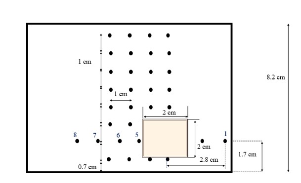
Figure 1: Schematic Representation of the Polystyrene in the Area
FIGURE 2
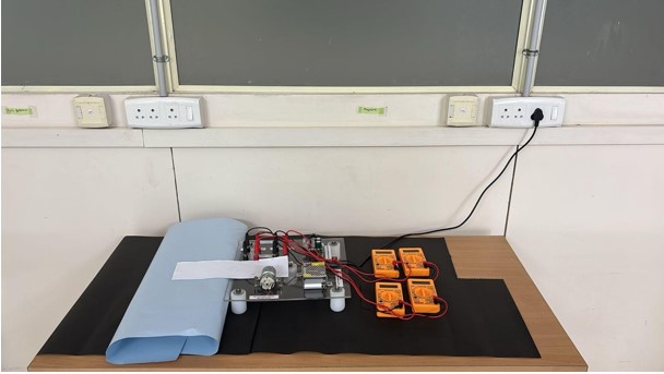
Figure 2: Experiment set up
FIGURE 3
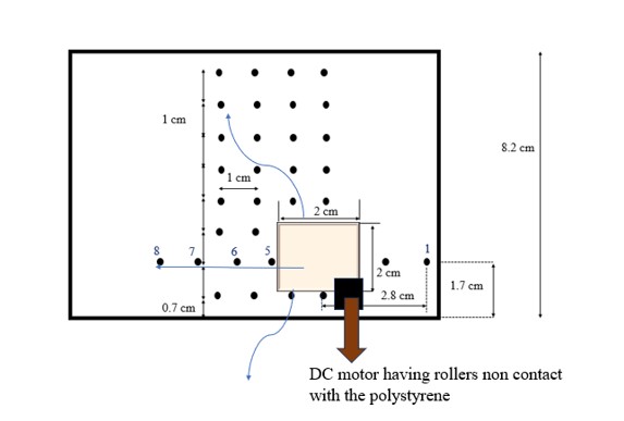
Figure 3: Schematics of Transport of Polystyrene with Time Under the Application of DC Motor Having Rollers. The Polystyrene Moves cm Distance for our Study.
FIGURE 4
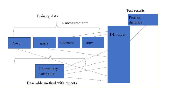
Figure 4: Network Architecture of the Data Driven Neural Network
FIGURE 5
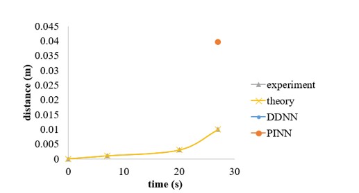
Figure 5: Comparison of Polystyrene Distance Traveled for P = 5.34 W. We have Experiments, Theory, DDNN and PINN Neural Networks
FIGURE 6
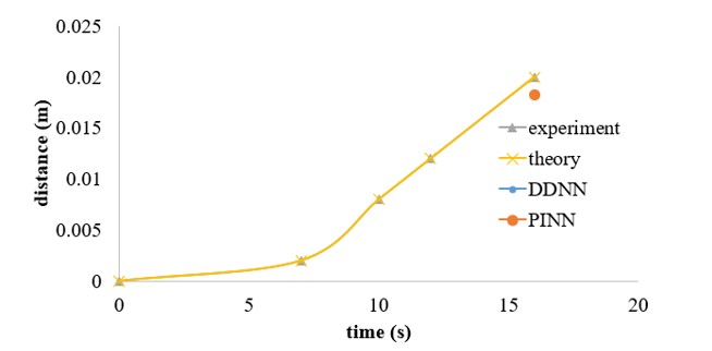
Figure 6: Comparison of Polystyrene Distance Traveled for P = 6.44 W. We have Experiments, Theory, DDNN and PINN Neural Networks
FIGURE 7
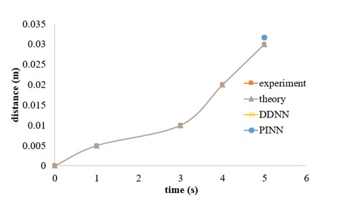
Figure 7: Comparison of Polystyrene Distance Traveled for P = 8.32 W. We have Experiments, Theory, DDNN and PINN Neural Networks
FIGURE 8
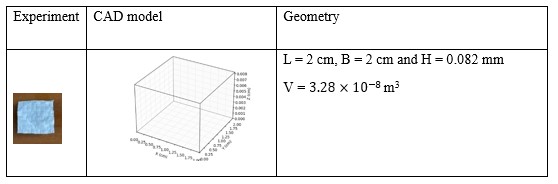
Table 4: Single Polystyrene Geometry, CAD Model and Image
FIGURE 9
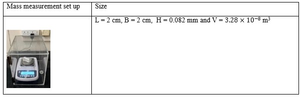
Table 5: Mass Measurement of Single Polystyrene. The Mass Balance is Protected with Acrylic Shield
Tables at a glance
Figures at a glance