Investigation of the Current–Voltage Characteristics of the DC Motor Having Rollers: Experiments and Neural Network Simulations
Received Date: February 16, 2026 Accepted Date: March 03, 2026 Published Date: March 11, 2026
doi:10.17303/jaist.2026.3.102
Citation: Nandigana V. R. Vishal (2026) Investigation of the Current–Voltage Characteristics of the DC Motor Having Rollers: Experiments and Neural Network Simulations. J Artif Intel Sost Comp Tech 3: 1-26
Abstract
In this paper, we perform experiments on DC motor having rollers. The motor are electrically wired to the components of switched mode power supply (SMPS), controllers and four digital multimeters. The multimeters are used to measure the voltage of the switched mode power supply and controllers. They are used to measure the current and the voltage of the motor. The device is mounted on the acrylic slab. The controllers are the logic component changing the DC voltage from 1 V to 8 V in the motor. We obtain the current from 0.64 A to 1.04 A, respectively. The power is in Watts. The voltage of the switched mode power supply is at 12.25V. The voltage of the controller is at 12.25 V. Further, we use data driven neural networks to match the experiments. We provide the experiment dataset to predict the current using neural network model. We develop physics from the theory informed in the neural network to predict the current. The accuracy of the model is good. Here, we develop physics from the partial differential equations informed in the neural network to predict current. The accuracy is good. Our model takes less simulation time. The training time is 20 s and predict time is 0.1 s.
Keywords: Artificial Intelligence; Machine Learning; Deep Learning; Materials and Engineering; Machines; Semiconductors
Introduction
The development of artificial intelligence (AI), machine learning (ML) and Deep Learning are going towards rapid revolutions for the machines to learn from the fields of mathematics, physics, materials and engineering. Relating the structure and shape of machines to their performance is an active area of research in deep learning. However, we do understand they work in sustainability over years from the relation between steel, machine and semiconductors. The shape of the natural elements to be in direct use with steel manufacturing is the future [1]. There is a research gap to relate the shape, mass, force to apply, force to repair, force on the machine with its mathematics. The manufacturing and mathematics should be precise. The generalized model from theory and partial differential equations are big research to know the machine manufacturing and its formula. Physics informed neural networks works best for the machine to train and predict its working. The dynamics of the machine are already known in the mathematics. However, interactions with multiple machines should be studied [2].
The quest to phase change on the machine interior or exterior forces and components then leads to further studies in hardware. The software provides the matching availability. The applications are available for area based manufacturing transport machines [3]. Machine learning is the simulation of the machines to give reliable results [4]. The sensors are used to provide the data. The sensors for the electrical machines are typical multimeters. They provide the current and voltage. The advanced sensors to know the formula of current are given. The partial charge of the materials are obtained. The multiple interactions of the machine are still nascent [5]. The classification of the partial charging with the materials and the neural networks are studied in detail [6-7]. Nowadays, the electrical machines are moving towards the study of energy, fuel, storage and electric vehicles technology. This ensures the multi domains engineering with the formula to predict the machine results and show the possibility for generalized model [8-12].
The hardware architecture in the electrical machines that provide the software neural network equivalent predict components are the controllers. The integration are new [13-19]. The load are the DC motor having rollers. The power of the motor is obtained sequentially [20-24]. There is scope for the future to integrate multi components that includes the electric wirings, their physics, insulators and lightweight materials [25]. The objective to provide generalized model to integrate with the physics informed neural networks and predict the machine integrated system works are necessary. The multi machines can provide the components that includes the light, digital electronics sensors, environment sensors, mass, pressure and force sensors [26-29].
In this paper, we study the device motor. We use switched mode power supply to provide the power to run the motor. We use controllers connected to the device. The controllers gives the necessary voltage to the motor. The digital multimeters are used to measure the voltage of the switched mode power supply. The multimeters are also used to measure the voltage of the controllers. We ensure the voltage of the switched mode power supply and controllers are the same. The multimeters are used to measure the voltage and the current of the motor. The system are mounted to the acrylic device. Here, we develop data driven neural networks to match the experiments. The model has good accuracy. We develop physics from the theory informed in the neural networks. We develop partial differential equations informed in the neural networks to match the experiments. The important contribution is the incorporation of experiment dataset with physics-informed neural networks. This is the novelty in our paper.
The rest of the paper is outlined as follows. Section 2 discusses the materials and methods. The necessary theory and governing equations are elucidated in Section 3. In Section 4, we provide the data driven neural network, physics from theory informed in the neural network and physics from partial differential equations informed in the neural networks. A detailed discussion of the current–voltage characteristics of the motor are given in Section 5. Finally, conclusions are presented in Section 6.
Materials and methods
Figure 1 shows the schematic set up of the device. The device consists of the components 1) switched mode power supply 2) controller 3) DC motor having rollers 4) electrical wirings 5) switch and 6) acrylic slab for the component mounting. The device set up are connected to measure the current and voltage of the motor. The measurements are taken using the digital multimeters. The voltage of the switched mode power supply and the controllers are also measured. The switched mode power supply have 12 V DC voltage. The switch is ON state to run the device.
The switched mode power supply, controller and the motor are purchased from Velonix, India. The switched mode power supply converts AC voltage to DC voltage. They have regulators that reduces the 220 V AC voltage to 12 V DC voltage. They have 7 wirings. The switched mode power supply have cuboid geometry outside (see Table 1). Inside there are semiconductor elements. The enclosure have 132 holes for environment safety and ventilations. The digital multimeter measures the steady state DC voltage of 12 V.
The geometry of the controller are cuboid in the box. They are not easy to measure. A controller is the feedback with electrical wirings. The voltage of the controller is measured. The controller controls the voltage and current of the load. Here, the motor is provided as the load. The electrical wirings with the controller and feedback network circuitry are well studied with many types of integration caps. The caps encapsulated to the wirings are typical insulators. The controller have components of semiconductor machined system, electrical wirings, insulation caps and feedback rotating knob. There are 8 wirings connected to the controller. The controller have a turning knob. The knob have 14 turns. Table 2 shows the relation between the knob and the corresponding voltage of the motor.
There are two external wirings to the motor. Table 3 shows the parameters of the motor.
The acrylic slab are fabricated in IITM. Table 4 shows the cuboid geometry parameters of the slab. The slab have 4 legs. They have internal wirings connected to the device.
The four multimeters are purchased from electronics, India. The 8 wirings from the multimeters are connected to measure the voltage of the switched mode power supply, controllers, motor and current of the motor. Figure 2 shows the experiment device. The switch is made in IITM.
Table 5 shows the geometry of the switch. The switch wirings are internal to the device. The switched mode power supply, controllers, motor, switch, electrical wirings, acrylic slab and multimeters are shown in Figure 2. The wind forces can cause small disturbances for the current measurements. They are the source of error. They are the environment conditions. The change in the current of the motor are negligible. The voltage readings on the motor, switched mode power supply and the controller do not change due to the wind forces. The multimeters are calibrated to measure the 12 V DC voltage of the switched mode power supply and 12 V of the motor as given by the manufacturer. The details are given earlier. Table 3 provides the parameters of the motor. We performed experiments from 1 V to 8 V using the controllers. We measured the voltage and current of the motor.
Theory
We calculate the charge inside the motor using Eq. (1).
where Q is the charge, C is the capacitance and V is the voltage of the motor. The charge and current relation are given in Eq. (2).
where I is the current and t is the time.
The capacitance of the motor is given in Eq. (3).
where ɛ0 = 8.854 × 10⁻¹² F/m is the permittivity of free space, ɛ r is the relative permittivity of the motor. L is the length and A is the cross section area of the motor. We assume the relative permittivity of the motor, ɛ r = 3. We measure the length L = 5.7 cm and calculate the area A = 5.3 × 10⁻⁴ m2. We take time t = 60 s.
Using Eq (1) to Eq (3) and fitting parameter α we obtain the current inside the motor. The fitting parameter α is used to match the experiments.
where α parameter are function of materials, distribution of materials, weight, concentration, moles, geometry, valence, constants, number of particles, oxidation reactions, electrical wiring, and device insulators. Table 6 shows the alpha values to model the current.
Armature current
We assume the armature shaft current and load current in the DC motor are equal. The armature current is calculated from Eq. (5)
where Iα is the armature current, P is the power and V is the voltage of the DC motor.
Armature Resistance
In this study we use the voltmeter-ammeter method. We lock the motor shaft to prevent rotation. We apply low voltage of 0.2 V to understand the DC motor having rollers do not rotate. The current is 0.61 A. The current is the armature current for the given 0.2 V. The armature resistance is calculated from Eq. (6)
where RA is the constant armature resistance for the DC voltage of 0.2 V and corresponding armature current (IA). Table 7 shows the low DC motor voltage and the corresponding armature current. The constant armature resistance is 0.32 ohm as shown in Table 7.
Back Electromotive force (EMF)
We use voltage equation method to obtain the back electromotive force. The back electromotive force is the magnetic effects in the DC motor. The back electromotive force is calculated using Eq. (7).
where Eb is the back electromotive force. We obtain the back electromotive force for different applied voltage from 1 V to 8 V. The armature current (Iα) for each applied voltage is obtained from Eq. (5). The power of the DC motor is given. The armature resistance (RA) is fixed to 0.32 ohm. The armature resistance is obtained as discussed earlier. Table 8 shows the back EMF for different voltage of the DC motor. Figure 3 shows the circuit diagram having the armature current, resistance and terminal voltage. The load DC motor is given. The back electromotive force is provided.
Angular velocity of the DC motor shaft
In this paper the maximum DC motor voltage is 12 V. At 12 V, the DC motor armature shaft rotates at 18000 revolutions per minute (rpm). The specification chart provides the rpm of the DC motor at 12 V. The angular velocity is calculated using Eq. (8).
where N is the speed of the shaft in revolutions per minute. Table 9 shows the speed and angular velocity of the shaft at 12 V of the DC motor.
Motor back electromotive force constant
The motor back electromotive force constant is calculated using Eq. (9).
where K e is the back electromotive force constant. K e is an intrinsic physical property of the motor. As discussed earlier we know the speed and angular velocity for applied voltage of 12 V on the DC motor. Using Eq. (9) we obtain the back electromotive force constant of 0.0064 V/(rad/s). The voltage is 12 V and angular velocity is 1884.96 rad/s. The back electromotive force constant K e is same for different voltage.
Relation between angular velocity and back electromotive force
The back electromotive force is related to the angular velocity of the motor using Eq. (10).
Here, we use the constant Ke = 0.0064 V/(rad/s) as discussed earlier. Table 8 gives the angular velocity of the motor for different back electromotive force. Eq. (8) is used to obtain the speed of the motor. Table 8 shows the speed of the motor in rpm.
Relation between Torque of the motor and armature current
The torque created by the motor is related to the armature current using Eq. (11).
where T is the torque of the motor. Table 8 shows the torque for different armature current. The armature current are calculated for voltage from 1 V to 8 V.
Governing equations
In this section we provide the partial differential equations to the motor. The device variables are provided in the simulations. The current of the motor are given in Eq. (12).
where S is the cross-sectional area of the motor, z is the valence and F is Faraday’s constant. The flux of the electrolyte is contributed by the potential gradient given by Eq. (13).
where D is the diffusion coefficient, c is the concentration of the electrolyte, φ is the potential, R is gas constant and T is the room temperature.
Substituting Eq. (13) in Eq. (12) and integrating over the cross section area we obtain the current in Eq. (14).
Here,
where E is the electric field, Lx is the length of the motor. The field equations Eq. (14) and Eq. (15) are solved to obtain the current. The current is given in Eq. (16).
Simulation Details
The length of the motor is LX = 5.7 cm. The diameter of the motor is 2.6 cm. The area is 5.3 × 10⁻⁴ m2. We study voltage from 1 V to 8V. The concentration, voltage and electric field of the device are provided in the Table 10. The diffusion coefficient of the electrolyte is D = 2 × 10⁻⁹ m2/s. We assume valence z = 1, Faraday constant F = 96485.3 C/mol and gas constant R = 8.314 J/ (mol K). Here, the room temperature T = 300 K. We consider 10 grid points. The voltage applied from the motor and its electric field are given in Table 10. The concentration assumed for each voltage are provided in the Table 10.
Data Driven Neural Network (DDNN)
Here we develop data driven neural network, physics informed from theory incorporated in the neural networks and physics informed from partial differential equations incorporated in the neural network. The neural networks to understand the experiment dataset are the novel contribution. We obtain the motor parameters that includes permittivity, gas constants, current, voltage and power, respectively. The simulation gives the applicability of early fault detection of insulation and degradation in the machine to relate with the specification chart. Table 11 shows the voltage and current of the motor. We performed four repeats. They are trial 1, trial 2, trial 3 and trial 4, respectively.
Figure 4 shows the schematic of the data driven neural network. The neural network uses training data. We consider 7 training data sets. The training data set 1 have variables [voltage, current and power] of the motor. The training data 1 was provided as a csv file. The variables are repeated 7 times giving [7× 3] values in each training data set.
Deep learning (DL) layer
We use ReLU rectified linear unit activation function in python. ReLU is a fitting function. The control theory provides the rectified linear unit. ReLU fits the variables. The model provides the weight for the training data. In our model the linear activation function are provided for maximum accuracy.
model = Sequential([
Dense(1024,activation='relu', input_shape=(Ny,)), Dense(1024, activation='relu'),
Dense(1024, activation='relu'),
Dense(Ny, activation='linear' )
])
model.compile(loss='mse', optimizer='Adam')
The model uses mean square estimation function to calculate the accuracy while obtaining the weight. The weight obtained are optimized with minimal loss. The code having the weight calculation in the python are given. The number of default lines 1024 are used to follow python software.
csv_logger = CSVLogger('training_log.csv', append=True)
model.fit(X_train, X_train, epochs = 200, batch_size = 30, callbacks=[csv_logger])
The epochs are studied. We find the epochs do not compromise the accuracy of the training data. The prediction for one test set data are studied. The model takes less computer time. The training time is 20 s and predict time is 0.1 s. The python code to predict the test variables are given.
testinput = []
Test = pd.read_csv('data/Test1.csv',header = None)
Test = Test.values testinput.append(Test)
testperforming = array(testinput).reshape(1, Ny) Simulation_time = np.zeros((1,1))
start = time.time()
testoutput = model.predict(testperforming, verbose=1) end = time.time()
Simulation_time.fill(float(end-start))
print("It took: ", Simulation_time, " seconds") AIoutput = pd.DataFrame(testoutput)
AIoutput.to_csv('Predict.csv',header = None, index = False)
The test data with the predicted variables of [voltage, current and power] are saved in the file.
Table 12 shows the training data 1 used in the data driven neural network. The training variables are [voltage, current and power].
Training data set 1
Table 13 shows the test data given to predict the test current from the data driven neural network. The test variables given are [voltage and power]. We provide 7 repeats of the test data to predict the test current 7 times using the data driven neural network.
Test set
Predicted results
Table 14 shows the comparison between the actual voltage and the data driven neural network. The residual and square of the residual are given. Table 14 shows the comparison between the actual current and the model. Table 15 shows the comparison between the power and the model.
We calculate the the root mean square error (RMSE). The root mean square error is calculated as given in Eq (10).
where Pi is the predicted value, Oi is the actual result for observation i. n is the number of data points.
The steps to calculate the root mean square error are given.
1. We first calculate the residuals (R). The residuals are obtained by calculating the absolute difference between the actual result and the predicted value. We avoid negative values in the answers because they are physical quantities.
2. We calculate the square of the residuals (R2).
3. We calculate the mean squared error (MSE). We sum and mean of all the square of the residuals, respectively. We consider n is the total number of data points.
4. We calculate the root mean square error by taking the square root of the calculated mean square error.
The mean squared error for the current is 0.08. The root mean square error is 0.28. The accuracy of predicted current from the data driven neural network are 72% compared to the experiments.
Physics from theory informed in the neural networks
Figure 5 shows the schematic of the physics informed from the theory in the neural network.. We consider 7 training data sets. The training data set 1 have variables [voltage, current and relative permittivity] of the motor. The training data are obtained from theory. The training data 1 was provided as a csv file. The variables are repeated 7 times giving [7× 3] values in each training data set.
The deep learning DL layer are same in the data driven neural network and physics from theory informed in the neural networks. The python lines of training code, fit function to obtain weights and predict lines of code use are same as mentioned in the earlier section. We provide 7 training data. We predict one test data. Table 16 shows the train data provided to the physics from the theory in the neural network. The training variables are [voltage, current and relative permittivity].
Training data set 1
Table 17 shows the test data provided to the neural network to predict the test current. The test variables given are [voltage and relative permittivity].
Test set
Predicted results
Table 18 shows the provided voltage and the physics informed theory in the neural network. Table 18 shows the comparison between the current and the model. We compare the relative permittivity in Table 19.
We predict the device variables including voltage, current and permittivity of the motor. The mean squared error for the current is 0.009. The root mean square error is 0.1. The accuracy of the model is good.
Physics informed partial differential equations in the neural network
Figure 6 shows the schematic of the physics informed from the partial differential equations in the neural network.. We consider 7 training data sets. The training data set 1 have variables [voltage, current of motor and gas constant]. The training data are obtained from partial differential equations. The training data 1 was provided as a csv file. The variables are repeated 7 times giving [7× 3] values in each training data set.
The deep learning DL layer are same in the data driven neural network and physics from partial differential equations informed in the neural networks. Table 20 shows the train data provided. The training variables are [voltage, current and gas constant]. Table 21 shows the test data set. The test variables given are [voltage and gas constant].
Training data set 1
Test data set
Predicted results
Table 22 shows the comparison between the provided voltage and the physics informed partial differential equations in the neural network. Table 22 shows the comparison between the current and the model. The residual and square of the residual for the current are given. The mean squared error for the current is 0.009. The root mean square error is 0.1. The accuracy of predicted current are good. Table 23 shows the comparison between the gas constant and the model.
Results and Discussion
Figure 7 shows the current-voltage characteristics of the motor. The intercept is 0.6. We understand the motor can use its current to drive light weight single and multiple polymers. Figure 7 shows the comparison of the current-voltage characteristics of the motor between the experiments, theory and simulations. The simulations shown in Figure 7 are from partial differential equations and the data driven neural networks. Figure 8 shows the comparison of the current-voltage characteristics of the motor between the experiments and physics informed neural networks. The physics is informed from the theory that is included in the neural network. Figure 8 shows the physics obtained from the partial differential equations that are included in the neural network. We observe when the model provided to the neural network is robust, the predict results for current match the experiments.
Table 24 shows the comparison of the current measured and the theory. The voltages are given. The mean squared error for the current is 1.85e-5. The root mean square error is 0.005.
Table 25 shows voltage, current from the experiments and the partial different equation numerical simulations. The residual and square of the residual are calculated. The mean squared error for the current obtained from the simulation is 0.00015. The root mean square error is 0.12.
Figure 9 shows the comparison between the test voltage of the motor with the data driven neural network. The mean squared error for the voltage is 0.08. The root mean square error is 0.28. We consider the root mean square error to obtain the accuracy. The accuracy is good.
Figure 10 shows the comparison between the power from the experiments and the data driven neural networks. The mean squared error for the power is 0.067. The root mean square error is 0.26.
Figure 11 shows the test voltage and the predicted voltage from the physics informed theory incorporated in the neural network. The mean squared error for the voltage is 0.008. The root mean square error is 0.1. The theory captures the physics of the device.
Figure 12 shows the comparison between the actual relative permittivity and the simulation. The relative permittivity is calculated for the motor. The simulation uses the physics from the theory incorporated in the neural network The mean squared error for the relative permittivity is 0.0012. The root mean square error is 0.04.
Figure 13 shows the voltage of the motor obtained from the experiments. We compare the test voltage in the experiment with the physics informed partial differential equation in the neural network. The mean squared error for the voltage is 0.06. The root mean square error is 0.25. We use physics from partial differential equations informed to the neural network. The field calculations are added to the neural network. The device variables are predicted using the simulations. The accuracy is good.
Figure 14 shows the comparison of the gas constant between the physics informed from the partial differential equations in the neural networks and the actual value. The mean squared error for the gas constant is 0.023. The root mean square error is 0.15. The multi domain device variables and the constants are obtained from our simulations.
Experiment Dataset parameters provided to Data Driven Neural network
Figure 15 shows the parameters of the device provided to the neural network. The architecture of the neural network are provided.
Train set
In this paper, we provide train set parameters that include voltage of the DC motor, armature current (same as the DC motor current), power of the motor, armature resistance, back electromotive force, back electromotive force constant, angular velocity of the motor, speed and Torque of the motor. We provide 7 training datasets. We provide the 7 training datasets in 7 csv files. We ensure each file have the parameters voltage of the DC motor, armature current (same as the DC motor current), power of the motor, armature resistance, back electromotive force, back electromotive force constant, angular velocity of the motor, speed and Torque of the motor. We ensure each file have the same parameters repeated seven times. Each csv file have [7× 9] array. Here the rows 7 are for repeats. The columns 9 are the parameters. Table 26 shows the train set experiment data sheet.
Test set
We consider 1 test set. The test set parameters include voltage of the DC motor, power of the motor, armature resistance, back electromotive force, back electromotive force constant, angular velocity of the motor, speed and Torque of the motor. We provide the 1 test set parameters in one csv file. We ensure the file have the parameters voltage of the DC motor, power of the motor, armature resistance, back electromotive force, back electromotive force constant, angular velocity of the motor, speed and Torque of the motor. We ensure the file have the same parameters repeated seven times. The one test csv file have [7× 8] array. Here the rows 7 are for repeats. The columns 8 are the experiment data sheet. The column of the current are filled with zero. Table 27 shows the test set.
The data driven neural network is used to predict the armature current for the test set parameters.
Predict current
Table 28 shows the predict current from the neural network. The predict current is 1.3 A. The experiment current is 1.04 A for voltage of 8 V. The accuracy is good. The variance is 0.0676. The root mean square error is 0.26. The variance and root mean square error are shown in Table 28. The neural network consistently reads the experiment data sheet, gets trained to predict the current for the test set parameters. The experiment data sheet is provided for DC motor device run by terminal voltage and controller. This is novel contribution of our paper.
Conclusions
To conclude, we measure the current-voltage characteristics of the motor. The experiments match the theory and simulations. We develop neural networks. We use theory in our neural networks to understand the benefits of physics in the device. We use partial differential equations in the neural network to understand the device. The model predicts the motor current with good accuracy. Our neural network predicts the motor current for experiment data sheet of the device. These robustness are significant contributions towards predicting the device variables. Our work can find applications in multi domain formula to experiments, energy, storage, manufacturing, robotics, packaging, material handling, semiconductors, electric vehicles and sensors.
Acknowledgments
There is no funding for this work.
Author Contributions
Nandigana V. R. Vishal: Conceptualization, Data curation, Formal analysis, investigation, methodology, resources, software, supervision, validation, visualization, writing – original draft, writing – review and editing.
Conflicts of Interest
The authors declare no conflict of interest.
Data availability
The data from the current study are available from the corresponding author upon reasonable request.
- A. Farea, O. Y. Harja, F. E. Streib (2024) Understanding Physics-Informed Neural Networks: Techniques, Applications, Trends, and Challenges, AI, 5: 1534-57.
- G. S. Misyris, A. Venzke, S. Chatzivasileiadis (2020) Physics-Informed Neural Networks for Power Systems, IEEE Power and Energy Society General Meeting, 1-5.
- Y. Fassi, V. Heiries, J. Boutet, S. Boisseau (2024) Towards Physics-Informed Machine Learning-Based Predictive Maintenance for Power Converters – A Review, IEEE Transactions on Power Electronics, 39: 2692–720.
- H. Wang, K. Ma, and F. Blaabjerg (2012) Design for reliability of power electronic systems, in Proceedings of 38th Annual IEEE conference, 33–44.
- A. Rauscher, J. Kaiser, M. Devaraju, C. Endisch (2024) Deep learning and data augmentation for partial discharge detection in electrical machines, Engineering Applications of Artificial Intelligence, 133: 1-13.
- E. Balouji, T. Hammarstrom, T. McKelvey (2022) Classification of Partial Discharges Originating From Multilevel PWM Using Machine Learning, IEEE Transactions on Dielectrics and Electrical Insulation, 29: 28 –94.
- G. Chianese, L. Iannucci, O. Veneri, C. Capasso (2025) Real-time estimation of battery SoC through neural networks trained with model-based datasets: Experimental implementation and performance comparison, Applied Energy, 389: 125783.
- C. Capasso, L. Iannucci, S. Patalano, O. Veneri, F. Vitolo (2024) Design approach for electric vehicle battery packs based on experimentally tested multi-domain models J Energy Storage, 77: 1-16.
- S. R. Daemi, C. Tan, T. G. Tranter et al. (2022) Computer-Vision-Based Approach to Classify and Quantify Flaws in Li-Ion Electrodes, Small Methods, 6: 2200887.
- D. Darbar, I. Bhattacharya (2021) Application of Machine Learning in Battery: State of Charge Estimation Using Feed Forward Neural Network for Na-Ion Batteries, ECS Meeting Abstracts, 02: 239.
- P. Dini, D. Paolini (2025) Exploiting Artificial Neural Networks for the State of Charge Estimation in EV/HV Battery Systems: A Review, Batteries, 11: 1-39.
- P. Pillai, S. Sundaresan, P. Kumar, K. R. Pattipati, B. Balasingam (2022) Open-Circuit Voltage Models for Battery Management Systems: A Review, Energies, 15: 6803.
- L. B. D. Giuli, A. L. Bella; R. Scattolini (2024) Physics-Informed Neural Network Modeling and Predictive Control of District Heating Systems, IEEE Transactions on Control Systems Technology, 32: 1182-95.
- F. Bonassi, M. Farina, J. Xie, and R. Scattolini (2022) On recurrent neural networks for learning-based control: Recent results and ideas for future developments, J. Process Control, 114: 92–104.
- S. Mowlavi, S. Nabi (2023) Optimal control of PDEs using physics-informed neural networks, J. Comput. Phys., 473: 111731.
- A. F. Guven, O. O. Mengi (2024) Nature-inspired algorithms for optimizing fractional order PID controllers in time-delayed systems, Optimal Control Applications and Methods, 45: 1251-79.
- A. Bonci, L. Longarini, S. Longi, G. Pompei, M. Prist (2025) Process regulation control using Echo State Networks: an ESN-based deep neural network approach for PID control, Procedia Computer Science, 253: 2369–76.
- M. Bolderman, M. Lazar, H. Butler (2021) Physics–guided neural networks for inversion– based feedforward control applied to linear motors, in Proceedings IEEE conferences 1115–20.
- J. A. Butterworth, L. Y. Pao, D. Y. Abramovitch (2012) Analysis and comparison of three discrete-time feedforward model-inverse control techniques for nonminimum-phase systems, Mechatronics, 22: 577–87.
- S. E. Hurt; H. A. Toliyat (2025) Physics Informed Neural Network Induction Motor Equivalent Circuit Parameter Estimation with Only Electrical Measurements, IEEE International Electric Machines & Drives Conference, 1081-6.
- S. Son, H. Lee, D. Jeong, K. Y. Oh, K. H. Sun (2023) A novel physics-informed neural network for modeling electromagnetism of a permanent magnet synchronous motor, Advanced Engineering Informatics, 57: 1-18.
- F. G. Ciampi, A. Rega, T. M. L. Diallo, S. Patalano (2025) Analysing the role of physicsinformed neural networks in modelling industrial systems through case studies in automotive manufacturing, International Journal on Interactive Design and Manufacturing, 1-11.
- K. Strantzalis, F. Gioulekas, P. Katsaros, A. Symeonidis (2022) Operational State Recognition of a DC Motor Using Edge Artificial Intelligence, Sensors, 22: 1-20.
- S. Yousefnejad, F. Bagheri, R. Alshawi, M. T. Hoque, E. Amiri (2025) Deep Learning Based Fault Detection Method in DC Motor Start, IEEE Transactions on Energy Conversion, 40: 1678–81.
- The Electric Wiring of Buildings, Nature, 126: 912, 1930.
- B.Gjorgiev, L. Das, S. Merkel, M. Rohrer, E. Auger, G. Sansavini (2023) Simulation-driven deep learning for locating faulty insulators in a power line, Reliability Engineering & System Safety, 231: 108989.
- J. Muller; K. Dietmayer (2018) Detecting Traffic Lights by Single Shot Detection, IEEE, International Conference on Intelligent Transportation Systems.
- R. Carvalho, Jorge Melo, R. Graça, G. Santos, M. J. M. Vasconcelos (2023) Deep LearningPowered System for Real-Time Digital Meter Reading on Edge Devices, Appl. Sci, 13: 1-13.
- A. Safonova, G. Ghazaryan, S. Stiller, M. M. Knorn, C. Nendel, M. Ryo (2023) Ten deep learning techniques to address small data problems with remote sensing, International Journal of Applied Earth Observation and Geoinformation, 125: 1-17.
FIGURE 1
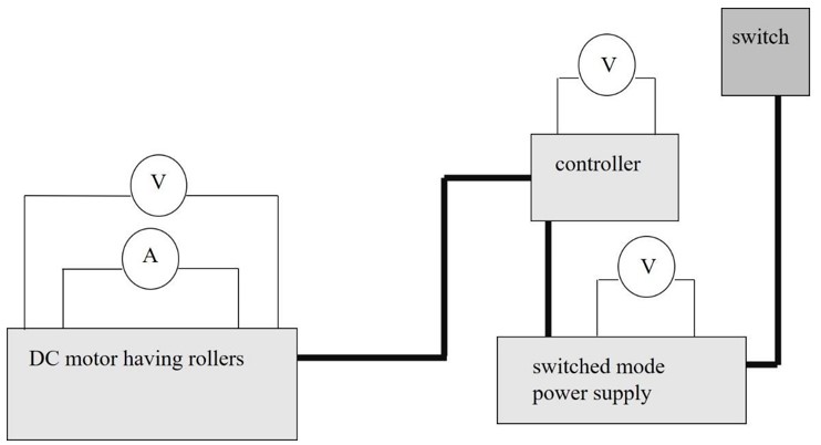
Figure 1: Schematic set up of the Device
FIGURE 2
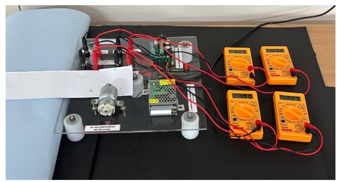
Figure 2: Experiment set up of the Device
FIGURE 3
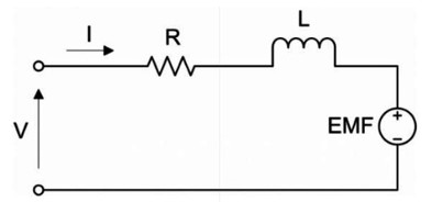
Figure 3: The Circuit Diagram Having the Armature Current, Resistance, Voltage, Load DC Motor and Back Electromotive Force
FIGURE 4
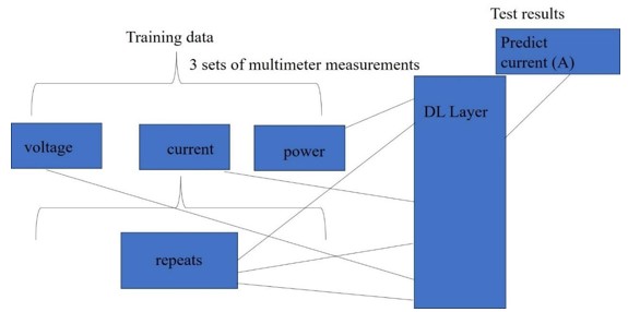
Figure 4: Schematic of Data Driven Neural Network
FIGURE 5
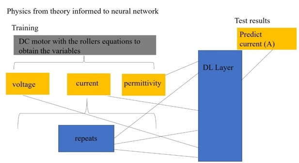
Figure 5: Schematic of Physics from theory informed in the neural network
FIGURE 6
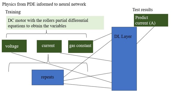
Figure 6: Schematic of Physics from Partial Differential Equations Informed in the Neural Network
FIGURE 7
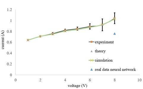
Figure 7: Comparison Between the Experiments, Theory and Simulations Current–Voltage Characteristics of the Motor. The Simulations Include Partial Differential Equations and Data Driven Neural Networks.
FIGURE 8
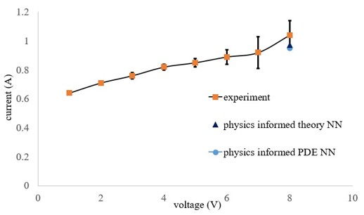
Figure 8: Comparison Between the Experiments and Neural Network Simulations of the Current– Voltage Characteristics. The Simulations Include the Physics from Theory Informed in the Neural Network and Partial Differential Equations and Data Driven Neural Networks. The Voltage of the Switched Mode Power Supply and Controller are Measured as 12.25 V in Our Experiments.
FIGURE 9
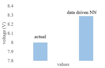
Figure 9: Comparison of the Voltage of the Motor Between Experiment and Data Driven Neural Network
FIGURE 10
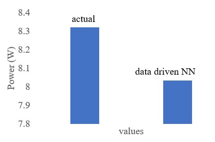
Figure 10: Power Obtained from the Experiments and Predict Results from Data Driven in the Neural Network.
FIGURE 11
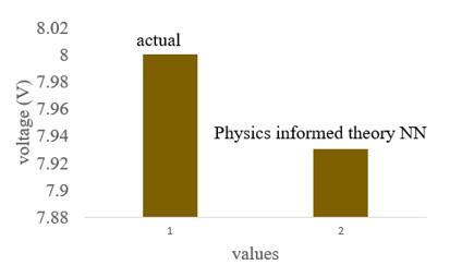
Figure 11: Comparison of the Voltage of the Motor Between Experiments and Physics Informed Theory in the Neural Network
FIGURE 12
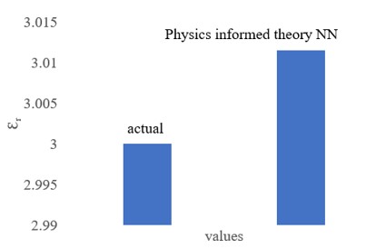
Figure 12: Relative Permittivity Prediction from Physics Informed Theory in the Neural Network
FIGURE 13
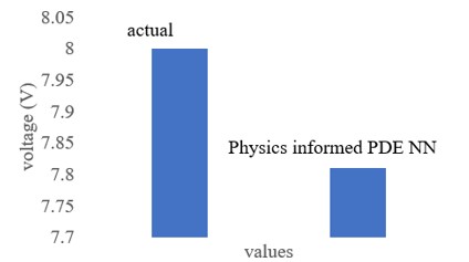
Figure 13: Comparison of the Voltage of the Motor Between Experiments and the Physics Informed Partial Differential Equation in the Neural Network
FIGURE 14
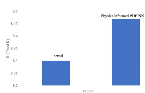
Figure 14: Gas Constant Prediction from Physics Informed Partial Differential Equation in the Neural Network
FIGURE 15
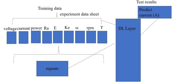
Figure 15: Schematic of Data Driven Neural Network for Parameters of the Device
Tables at a glance
Figures at a glance