Tables at a glance

Table 1

Figures at a glance

Figure 1

Figure 2

Figure 3

Figure 4

Figure 5

Figure 6

Figure 7

Table 1

Diameter	1 mm	2 mm	3 mm	4 mm	5 mm
RC	0.10	0.60	0.89	0.96	0.92

Table 1 : Recovery coefficients from the image quality phantom

FIGURE 1

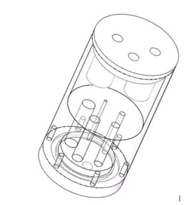
Figure 1: The schematic diagram of the NEMA image quality phantom

FIGURE 2

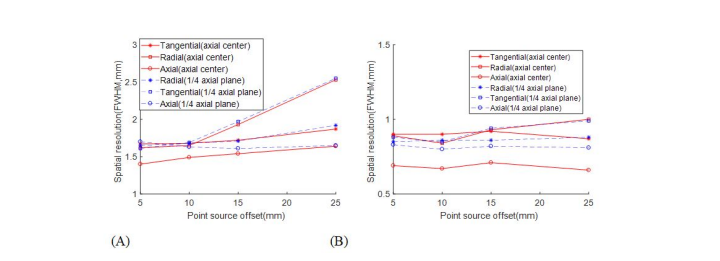
Figure 2: Spatial resolution results for: (A) FBP, (B) OSEM+PSF

FIGURE 3

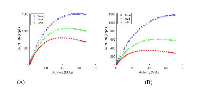
Figure 3: Results of Noise Equivalent Count Rate experiments for: (A) mouse-like phantom, (B) rat-like phantom

FIGURE 4

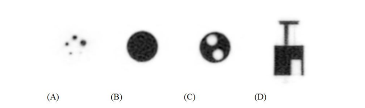
Figure 4: Reconstructed image of the NEMA image quality phantom: (A) a transverse slice of the 1, 2, 3, 4, 5 mm hot-rod regions; (B) a transverse slice of the uniform region; (C) a transverse slice ofthe cold region containing water and air; (D) a coronal slice of the phantom

FIGURE 5

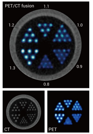
Figure 5: Images of the Micro Derenzo phantom. Top: PET/CT fused images; bottom-left: CT image; bottom-right: PET image

FIGURE 6

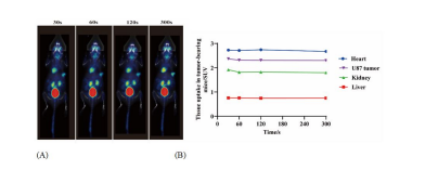
Figure 6: Micro PET/CT images of U87 tumor-bearing mouse with various acquisition durations 1 h after 18F-FDG (68 μCi) intravenous injection: (A) Coronal sectional images of tumor site with scan time of 0 - 30 s, 31 - 60 s, 61 - 120 s, and 121 - 300 s, respectively; (B) Time activity (SUV-mean value) curves of the heart, liver, kidney and tumor of the U87 tumor-bearing mouse

FIGURE 7

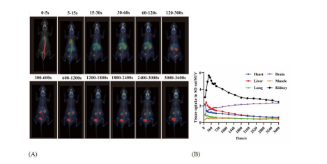
Figure 7: Dynamic PET/CT images of a SD rat after administrated with 40 μCi 18F-FDG:(A) Maximum intensity projection (MIP) fused PET/CT images with frames of 0 – 5 s, 5 - 15 s, 15 - 30 s, 60 - 120 s, 300 - 600 s, 600 - 1200 s, 1200 - 1800 s, 1800 - 2400 s, 2400 - 3000 s, 3000 - 3600 s; (B) Time activity curves of the heart, brain, liver, muscle, lung and kidney, derived from the reconstructed dynamic images of various acquisition times