Most physical and chemical processes encountered in chemical and process engineering often lead to differential equations which are as varied as the complex mass, momentum and energy transport processes they represent. Thus finding/selecting the appropriate one to use in any given situation is not an easy task. Following the realization that the solution of any differential equation can be generally expressed as a polynomial (truncated power series) which can be regressed by the least square method, and the coefficients of the regressed model linked to that of the binomial formula led to a generalized computational procedure for solving a wide-range of differential equations in chemical and process engineering (both initial and boundary value problems). The method was found to be computationally efficient and inexpensive as it is fast converging and free from rounding off errors and overshoot.

Keywords: Physical and chemical processes; Differential equations, initial and boundary value problems; least square regression analysis; binomial formula; computational procedure

Differential equations-used in most science and engineering analysis- are particularly important in modeling chemical engineering systems. As the physical and chemical laws governing these processes (heat, mass, and momentum transfer) are complex, as well as the chemical reactions, reaction heat, adsorption, desorption, phase transition, multiphase flow, etc,associated with them, so also are the differential models arising from them and include:, homogeneous/non-homogeneous, linear/non-linear , constant/variable coefficients, 1^st, 2^nd or higher orders, and systems of simultaneous differential equationsboth for Ordinary and partial differential equations. Numerous methods have been developed for solving them. They include:

Exact methods such as Method of undetermined coefficients, Integrating factor, Method of variation of parameters/separation of variables[1,2].

Approximate (but convergent) methods such as Successive Approximations, Perturbation Theory, Multiple scale Analysis, power series solutions, Generalized Fourier series/orthogonal functions [3].

Numerical methods such as: Euler methods; Trapezoidal rule; Runge–Kutta methods; Finite difference methods ;Finite element methods, gradient discretisationmethods[4-18].

Numerical techniques are particularly important since most realistic deferential equations in chemical and process engineering do not have exact analytic solutions, therefore, approximate/numerical techniques, such as Runge-Kutta, Euler, Newton gradient methods, finite difference/element) are used extensively.These methods have proven rather successful in dealing with both linear and nonlinear problems as well as initial boundary problems(IVP) and boundary value problems(BVP). Despite these obvious advantages, they have some demerits. Since they involve discretization, they have rounding off errors and are computationally expensive, and in some cases will not converge to the true solution.

particular generalized procedure which is used to grind most differential equations is the Power Series Method(PSM) (https://www.researchgate.net/publication/293652327). This method has proven rather successfulin dealing with both linear as well as nonlinear problems, as it yields analytical solutions andoffers certain advantages over standard numerical methods. It is free from rounding off errorssince it does not involve discretization, and is computationally inexpensive. In spite of the advantages of PSM, it has some drawbacks, the major one being that it cannot handle boundary value problems, as it can only handle initial value problems.Thus finding/selecting the appropriate one to use in any given situation is not an easy task.

In this article, we present a more generalized computational approach, which is amodification of PSMusing the Binomial formula/least square approximation, the goal being to use the same platform/ procedure tosimulate all differential equations in chemical and process engineering(both initial and boundary value problems),and to overcome the shortcoming of other methods.

Usually we solve differential equations to obtain the value of the dependent variable in terms of independent variable/s, which are finally represented in graphs for better visualization and analysis. These solution curves are as varied as the differential equations they are representing. Thus the first step in unification/generalization is to find a general expression that can fit all data/graphs as accurately as possible. We know from statistics that any set of data (or expression) can be regressed by the general least square method [19,20], and generally, the higher the order of the regression, the more accurate the solution becomes.Thusto fit an appropriate equation to the data, we use regression analysis given generally as:

Y = a0 + a1X + a2X² + a3X³ + … + anXⁿ(1.1)

The coefficients , ai , are found by least square method, applied to the X-Y data,which results in the matrix:

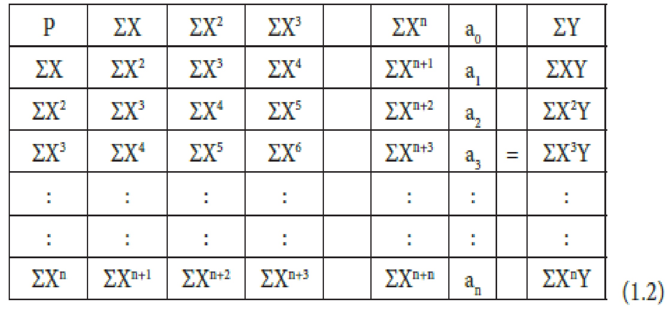
Similarly the solution of any differential equation can be expressed and regressed as a polynomial of the eq.1 form.Notice that polynomials are simply finite or truncated power series. That is a polynomial is a power series where the coefficients, ai beyond a certain point are all zero. Thus the coefficients of the polynomial can be found by manipulating power series by differentiation and theuse the Taylor series expansion. These manipulations will lead to a recurrent relation- recursion equation- given as:

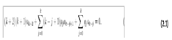
The above equation is called a recurrence relation for the coefficients of the power series. For instance the first three equations of the relation are:

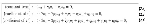
Hence, once the first two coefficients, a0 and a1, are known(which are actually the initial boundary conditions) then all other coefficients are determined by the recurrence relation. Thus PSM is limited to only initial boundary value (IVP) problems as it cannot handle boundary value problems (BVP) because of its recursive nature. In a nutshell, the method admits a polynomial expression as the solution of the differential equation, which when differentiated and substituted into the differential equation gives a recurrence relation-recursive formula, which by knowing the initial boundary conditions, gives the coefficients of the polynomial expression, hence the solution of the differential equation. This approach is adopted, with some modifications, in solving differential equations(both initial and boundary value problems). All that is needed is to find the right order and the right parameters(coefficients) of the polynomial expression(representing the differential equation); by modeling/numericalanalysis as this work shows.

Let us start with a general second order linear ODE with both constant and variable coefficients as follows:

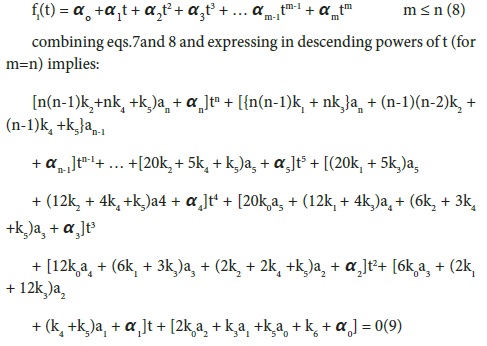
f_i(t) can be any function of t namely: linear, nonlinear, exponential, trigonometric,Logarithmic, or their combinations. Whatever the form or forms of f(t), the general procedure is to remodel and express in terms of polynomial expressions within the solution interval, using the least square regression analysis already explained. Thus:

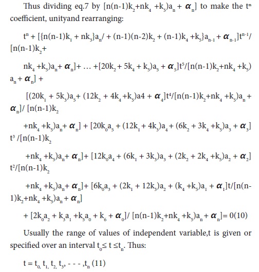
therefore t - t₀ = t- t₁ = t- t₂ = t- t₃ = … = t-t_n = 0 (12) This implies that: t –t_i = 0_i= 0,1,2,3…,n(13) Thus (t - t_i)ⁿ = 0t₀≤t_i≤t_n (14)

Eqs. 10 and 14 are equivalent. This realization/discovery that eqs.10 and 14 are equivalent is the key to new computational method for generalization of the method of simulating differential equations (both IVP and BVP). Thus the parameters or coefficients of eq,14 are linked to those of eq.10using binomial formula:

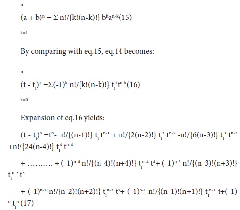
Thus eq.17 and eq.10 are equivalent, and term by term comparison result in the following equations that linked their coefficients:

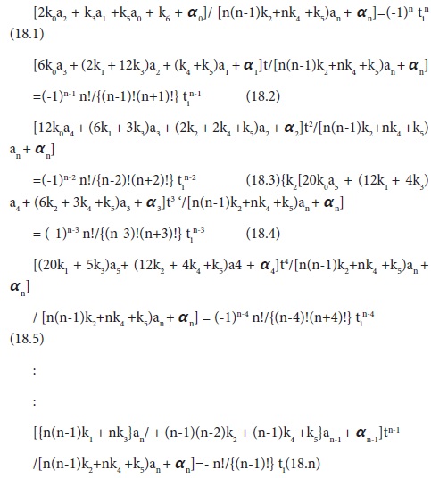
Thus there are n-equations (eqs. 18.1 to 18.n) with n+1 unknown parameters, a₀,a₁,a₂,a₃,a₄,a₅,…,a_n thereby requiring additional equation/s, which are found from the boundary conditions of the problem. Usually the boundary conditions can be one( for IVP of first order) or two ( for BVP of first order and IVP/BVP of second order). Let us consider the two cases, and clearly visualize the procedures by considering n=5. Thus for n=5, eq.18 set reduces to:

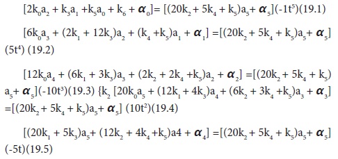
Thus we have five equations (eq.19.1 to 19.5) with six unknowns (a0 to a6). The remaining equation/s will come from the boundary conditions as follows:

Case 1: One point boundary value problem. for 1st order IVP, whereY(τ) is given, thereby giving one boundary equation, eq.4 in terms of the boundary condition provides the remaining equation(for n=5) as:

Y(τ) = a0 + a1τ + a2τ² + a3τ³+ a4τ⁴ + a5τ⁵ (19.6)

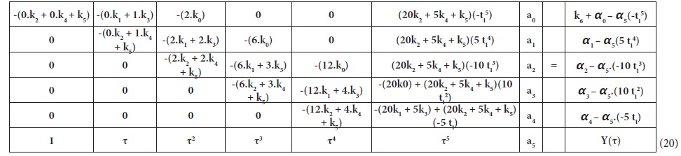
Rearrangingeqs. 19.1 to 19.6 result in the following sample simulation matrix for one point IVP ODE’s:

Case 2: Two points boundary value problem.

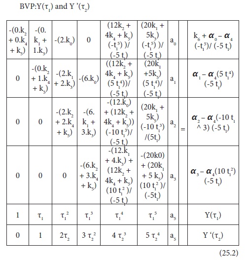
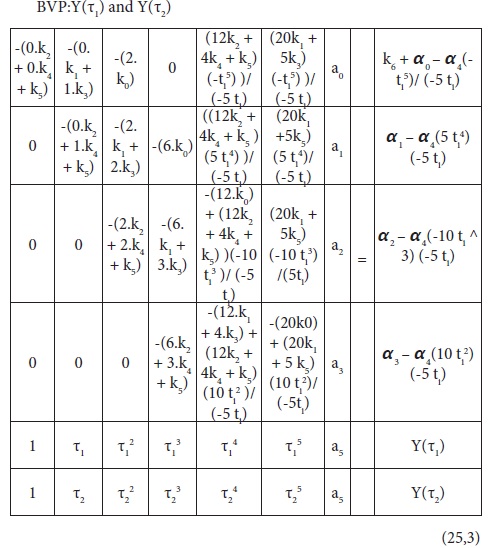
Similarly for BVP of first order ODE or both for IVP and BVP of second order ODE,s where Y(τ) and Y’(τ)or Y(𝞽1)and Y’(𝞽2) or Y(τ1) and Y(τ2) pairsare given, thereby given two boundary equations in each case as follows:

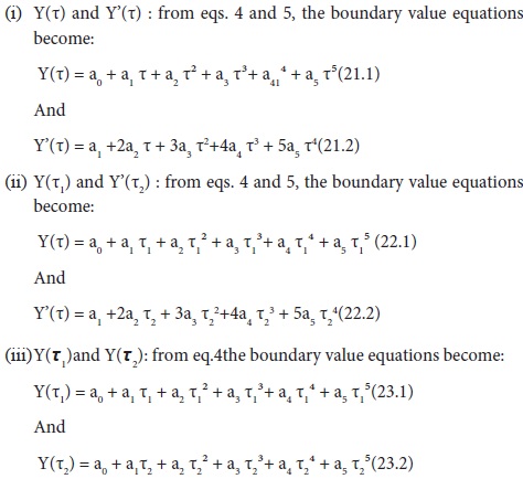
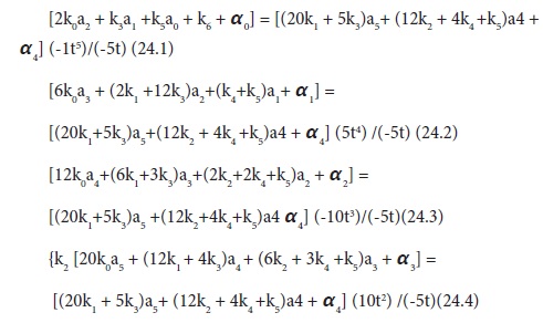
This implies we now have five-main equations(eqs.19.1 to 19.5) and two boundary equations (eqs. 21.1 and 21.2 or 22.1 and 22.2 or 23.1 and 23.2) with only six parameters (a0,a1,a2,a3,a4 and a5). Thus we need to reduce the main equations from n=5 to n-1=4 to accommodate the two equations from the boundary conditions. Thus eqs.19.1 to 19.4 are divided by eq.19.5 to give the required four equations as follows:

Rearranging and combining eqs.24.1 to 24.4 with the boundary value equations result in the following sample simulation matrix in each case as follows:

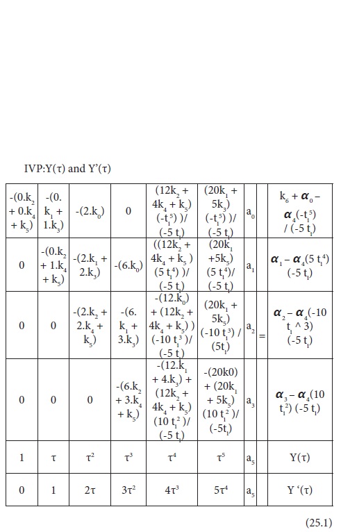
A closer observation on the sample simulation matrices show certain similar trends that can lead to generalization and extension to higher order and matrix size. Thus a spreadsheet program has been developed by the authors for handling higher order ODE’s and matrix size.

The analyses here follow the same pattern as the linear case explained in the previous section. Thus let us illustrate by converting the general second order linear ODE of eq3 into second order non linear form by making the y-coefficientvariable in the dependent variable as highlighted in eq.26:

(k0+k1t + k2t2)d2Y/ dt2 + (k3+k4t) dY/dt + (k5 + k6Y) Y + f(t) + k7 = 0 (26)

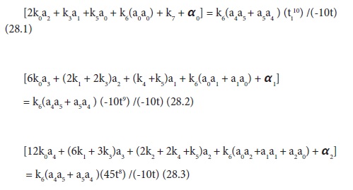
Eq.26 is a second order nonlinear ODE. Thus by following similar regression procedure as explained in the linear cases, the resulting equation(for the sample case of n=5) is:

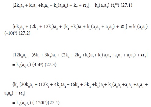
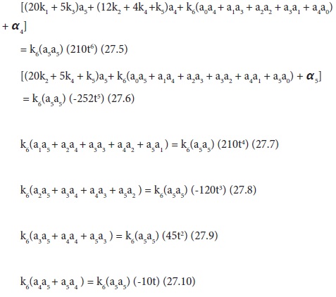
Thus we have ten equations(eqs. 27.1 to 27.10) with six unknowns(a0---a5). Boundary conditions will also supply more equations. For instance two boundary conditions will add additional two equations, making a total of twelve. Following the usual procedure, we need to modify eq. 27 set so as to match the number of unknowns. Instead of merging /combining, we need to adopt a less cumbersome and easily programmable technique of defining new variables so as to match the number of equations.Thus by dividing eqs. 27.1 to 27.9 by eq. 27.10 followed by dividing eqs. 27.6 to 27.10 only with a5a5 and defining c₅ = a₅/a₅ ,c₄ = a₄/a₅, c₃ = a₃/a₅, c₂ = a₂/a₅ , c₁ = a₁/a₅,c₀ = a₀/a₅,eqs. 27 set now becomes:

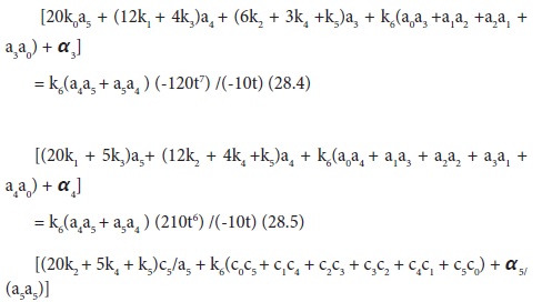
Thus with these transformations, we now havenine equations with twelve unkonws (a0 to a5 and c0 to c5) remaining three more equations to complete, which is supplied by the two boundary equations and the identity: c5 = 1. Eqs.28 set are non linear algebraic equations, which can be solved by successine iterations or by newtons gradient methods via matrix algebra. Once again close observation shows trends that can lead to generalization to any order and matrix size.

Let us illustrate the procedure by considering two simultaneous first order ODE’s with constant coefficients as shown:

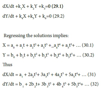
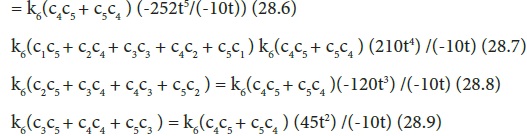
inserting eqs.29to 32 into eq.28 set , expanding and marching term by term with the corresponding modified binomial coefficients leads to the following equations ( for n=5):

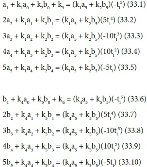
Note that ti’ are the values of the independent variable at the solution interval specified. Thus we have ten linear equations with twelve unknowns (a0 to a5 and b0 to b5), thus requiring two additional equations to complete. These are supplied by the boundary conditions of the problem. For the IVP where X(0) and Y(0) or X(𝞽) and Y(𝞽) are given, thus providing additional two equations, hence no modifications are needed in the eqs.33 set. However for BVP where the equations are more than two, we need to make modifications in the eqs.33 set to accommodate all the boundary value equations, as exhaustively explained in the previous sections. Thus eqs.33 set along with the boundary value equations are solved via matrix algebra to give the solutions of the systems of ODE, that is X and Y in this case. The sample matrix is shown below (for IVP).

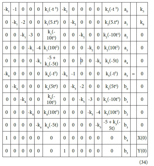
A closer look at the matrix equation shows trends that can lead to generalization to any matrix size. Higher orders and variable coefficients and non linear forms are equally handled as previously explained.

In this section, some chemical engineering applications are given to demonstrate the accuracy, efficiency and generality of the present method.

Let us consider an unsteady continuous flow, well stirred mixer as shown in Figure 1

It is desired to find the concentration profile of the salt in the tank. The governing differential model is:

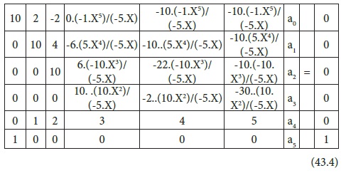
dC/dt + 3C/(60 +2t) =0.5 , C(0) =10 (35)

We will use this example to illustrate the procedure for the new method. Equation 35 is rearranged in the general linear ODE format (eq.3) to give:

(60 +2t) dC/dt + 3C - t- 30 = 0 C(0) =10 (36)

This is a first order one point IVP problem(Y(0) given) of the simulation matrix type, eq. 20, thus term by term comparison of eq.37 with the general linear ODE standard expression (eq,3) implies; k0=0, k1=0, k2=0, k3=60, k4=2, k5=3, 𝞪1 = -1, k6 = -30, thus substitution of these k-values along with the boundary values into the simulation matrix(eq.20) results in the matrix

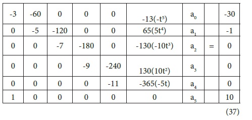
Thus for different values of t in the solution interval specified, in this case 0 ≤ t ≤ 15; the matrix is evaluated for the parameters, ai, from where the corresponding values of C(t) is found.

eg. For t= 15, the matrix (eq.37) becomes:

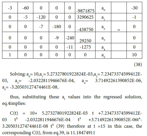
Similar procedure is repeated for the next matrix size (n=6) and for higher matrices until convergence.

let us consider an example of diffusion and first order chemical reaction in a catalystslabFigure 2(Rice and Do, 1995)

The second order differential model and the boundary conditions are:

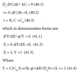
This is a first order boundary problem, (Y(0) given) of the simulation matrix type, eq. 25.2, thus term by term comparison of eq.37 with the general linear ODE standard expression (eq,3) implies; k0=1, k1=0, k2=0, k3=0, k4=0, k5= -100, 𝞪i = 0, k6 = 0, thus substitution of these k-values along with the boundary values into the simulation matrix(eq.20) result in the matrix:

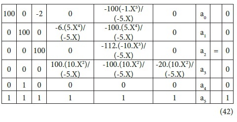
let us consider an elementary second order differential equation:

d2y/x2-2dy/dx - 10y = 00 < x < 1 (43.1)
x = 1 ;dy/dx =0, (43.2)
x = 0; y =1 (43.3)

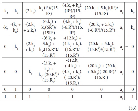
This two point BVP can be used to describe a chemical reaction occurring in a fixed bed.Since this a two point boundary problem, simulation matrix eq.25.2 amd its higher forms are used, with the eq.43.1

parameters in comparison with the general form, (eq,3) becoming; k0=1, k1=0, k2=0, k3=-2, k4=0, k5= -10, 𝞪i = 0, k6 = 0, thus substitution of these k-values along with the boundary values into the simulation matrix(eq.25.2) result in the sample simulation matrix for n=5:

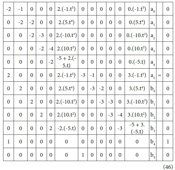
Let us consider a constant volume batch reactor undergoing the series the reaction sequence:

k ₁ k₂
A→B → C

For a first order kinetics, the differential equations describing the process are:

dC_A/dt =-k₁C_A (44.1)
dC_B/dt = k₁C_A – k₂C_B (44.2)

By including the coefficients and rearranging in standard format (eqs.28 set), eqs.44 set become:

dC_A/dt+2C_A = 0 (45.1)
dC_B/dt -2C_A + 3C_B = 0 (45.2)

and term by term comparisons implies: k₁ = 2, k₂ = 0, k₃ = 0, k₄ = -2, k₅ = 3, k₆ = 0; thus substitution of these k-values along with the boundary values into the simulation matrix (eq.34) and its extensions, result inthe sample simulation matrix for n=5:

Let us consider a second order chemical reaction in a plug flow reactor(with no axial dispersion) as shown in Figure 3 (Rice and Do, 1995).

Thus the nonlinear differential model governing the formation of a product(with no axial dispersion ) is as follows

udC/dz = kC² z= 0; C =C₀ (47)

where k=1; u=1 and C₀=1 ;0 ≤ z ≤ 0.9

rearranging in standard format of eq.26 implies:

udC/dz - kC²= 0 (48)

Thus term by term comparison of stabdard nonlinear eq.26 with eq.48 implies: k₀ =0; k₁=0; k₂=0; k₃=1; k₄=0; k₅ =0; k₆=-1; f(t) =0; k₇= 0

To illustrate the new procedure, eq.48 is a non linear first order differential equation.Thus using eq.27 set and following the usual procedure, the nonlinear ODE is solved using Newton’s gradient method.

Finally, let us consider an important problem in chemical engineering: to predict the concentration profile for a diffusion andreaction in a porous spherical catalyst pellet, hence the overall reactionrate of the catalyst pellet. The variable coefficient differential model is:

D [ 1/r² d/dr( r² dc/dr ) ] =k f(c) , 0 < rp (49)

where
r = radial coordinate (r_p= pellet radius)
D = diffusivity
c = concentration of the given chemical specie
k = rate constant
f(c) = reaction rate function
with
dc/dr = 0 at r = 0 (symmetry about the origin)
c = c₀ at r = r_p(concentration fixed at surface)
for an isothermal first order case, eq.50;in dimensionless form becomes:
d²C/dR² + 2/R dC/dR =φ² C;0 < R < 1 (50)
with the boundary conditions:
dC/dR=0 at R =0 (51.1)
Where thele modulus, φ, is :
φ = r_p(k/D)^1/2(51.3)
To simulate with the new generalized procedure, eq. 50 is first arranged in standard format as follows:
R d2C/dR2 + 2 dC/dR -φ2 R C = 0 (52)
For the case where φ=2.236, the coefficients are k₀ = 0; k_{1/sub> = 1; k2 = 2; k3 = 0; k4 = 0; k5 = -(2.2362); k6 = 0; k7 = 0; and the sample simulation matrix (n=5) becomes:}

Thus substituting the values of k’s and solving the matrix eq,53 and the corresponding higher matrices within the solution interval, until convergence.

Thus in all the above cases, the matrixes are evaluated for the coefficients, ai’s from where the solution of the ODE,Y is found by substituting into eq.4. The procedure is repeated for higher matrices until convergence, that is when there is no more significant different between the values ofY for two adjacent matrices, signifying the solution of the differential equation.All calculations are carried out by the spreadsheet programs developed by the authors.

Table 1Table 2,Table 3,Table 4,Table 5,Table 6show the results of the new method for varying chemical and process engineering applications. As observed, the new method gave the accurate results when compared with the exact (analytical) solutions, as can be seen from the absolute error, which is the absolute difference between the new method and the actual solution. Furthermore, the convergence is faster, since generally the solution converges on or before the matrix size, N=45, as compared with other numerical techniques (Table 7), which requires much higher matrix/grid size, N to get closer to the actual solution.Finally the general convergence sequence of the new method, shown in Table 8 and illustrated in figure 4 ensures that the method always converges to the solution, and does not have problems of overshoot andis free from rounding off errorsencountered in the other methods. Above all the new method is a generalized approach since as can be seen; a wide-range of chemical and process engineering problems are solved using the same procedure/platform.Thus the new method is efficient, computationally inexpensive, accurate and general.

In this work, a new generalized computational technique was developed (and illustrated) for solving differential equations (both initial and boundary value problems) in chemical and process engineering. This follows the realization that any differential expression can be regressed by the least square method and the coefficients of the regressed model linked to that of the binomial formula. Thus a generalized simulation matrix was developed for solvinga wide-rangedifferential equations of any order and forms. Both initial and boundary value problems are treated using the same procedure, so also are the differential models arising from them and include:, homogeneous/non-homogeneous, linear/non-linear , constant/variable coefficients, 1st,2nd or higher orders, and systems of simultaneous differential equationsboth for Ordinary and partial differential equations.In this first publication, ordinary differential equations were illustrated. In subsequent articles, we extend the new method to partial differential equations.