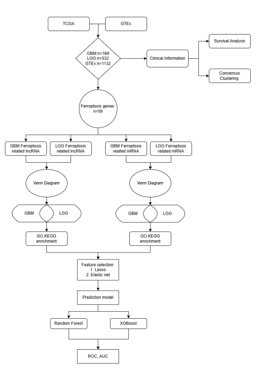
Figure 1: Workflow of this study

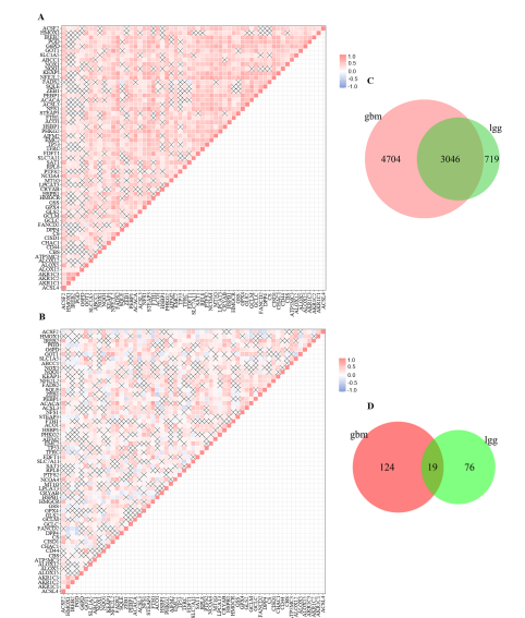
Figure 2: Correlation of ferroptosis-related genes in pairs and Venn diagrams for ferroptosis-related genes. (A-B) Heatmap of the correlation of ferroptosis-related genes in GBM (A) and LGG (B), respectively. Only pairs with correlation and t-test with p< 0.05 were shown; (C) Venn diagram of mRNAs related to ferroptosis genes that the filtering condition is |cor| > 0.7, p < 0.001; (D) Venn Diagram of lncRNAs related to ferroptosis genes that the filtering condition is |cor| > 0.7, p < 0.01.

Figure 3: Gene expression difference of ferroptosis-related genes in GBM and LGG. (A) A boxplot demonstrates the gene expression level between GBM and LGG in each ferroptosis-related gene; (B). Heatmap of expression difference in GBM and LGG combined with clinical information of patients.

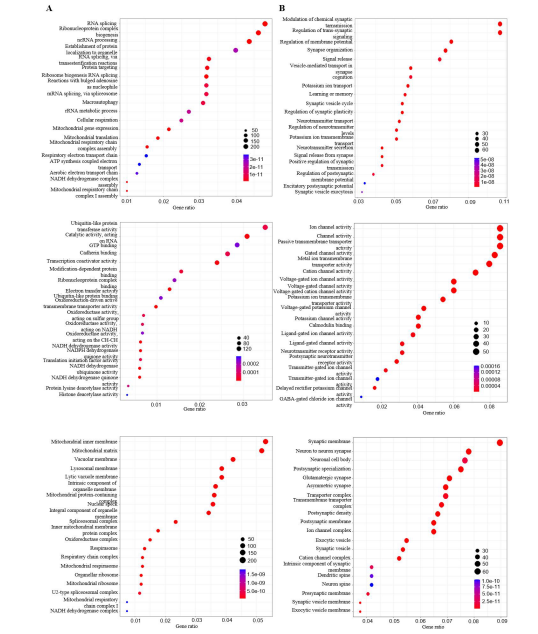
Figure 4: Performed GO functional analysis on mRNAs from GBM and LGG. (A) Top: GO analysis on biological process on ferroptosis-related mRNAs in GBM. A few of the biological processes were focused on mitochondrial functions. Middle: GO analysis on molecular functions, and a great amount of functions were focused on oxidoreductase activities. Bottom: GO analysis on cellular component functions, the main functions in this plot were involved with mitochondrial again; (B) Top: GO analysis on ferroptosis-related mRNAs in LGG. GO analysis on biological process that most functions were about chemical synaptic transmission. Middle: GO analysis on molecular functions, and a lot were chemical channel activities. Bottom: GO analysis on cellular component functions, and many functions were about synaptic activities.

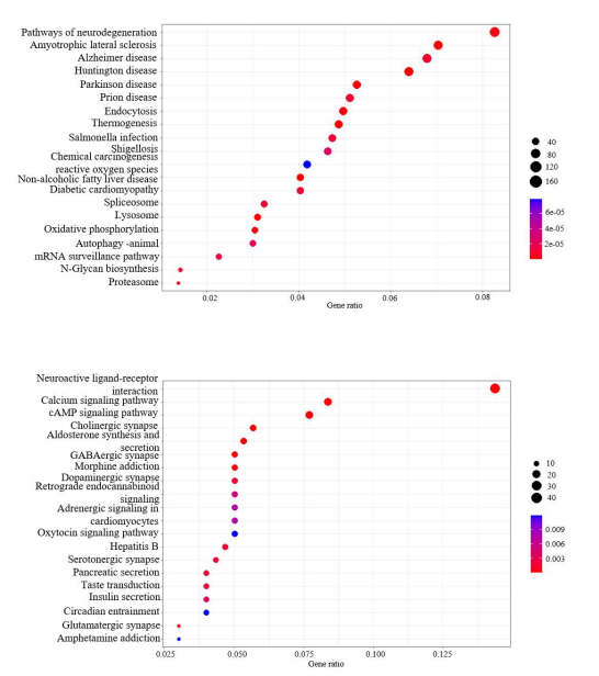
Figure 5: KEGG analysis in GBM and LGG. (A) The KEGG pathway enrichment analysis for exclusively expressed mRNAs in GBM; (B)The KEGG pathway enrichment analysis for exclusively expressed mRNAs in LGG.

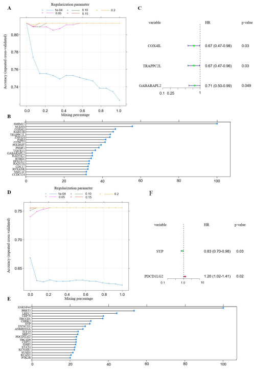
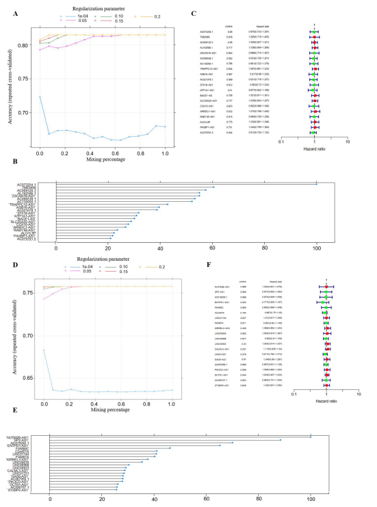
Figure 6: Parameters of feature selection using elastic net. (A) The plot showed the changes in accuracy when the algorithm took in diffrent values of regularization parameter where the blue dotted line represented a series of parameter that was equally cut between 1e-04 to 0.05, the same to all the other lines; (B) The variable importance of the features selected by elastic net after we obtained the optimal value from previous plot. (C) The forest plot of the 20 selected ferroptosis-related mRNAs and ran them into survival analysis, only three genes showed survival related and both lncRNAs had HR less than 1; (D) The plot of the changes in accuracy when the mixing percentage changed at different value of regularization parameters;(E)The top 20 ferroptosis-related mRNAs in LGG that were selected from elastic net, and ranked with variable importance; (F) The two mRNAs among the 20 selected variables that were survival related, and SYP had the HR less than 1 whereas the HR of PDCD1LG2 was greater than 1.

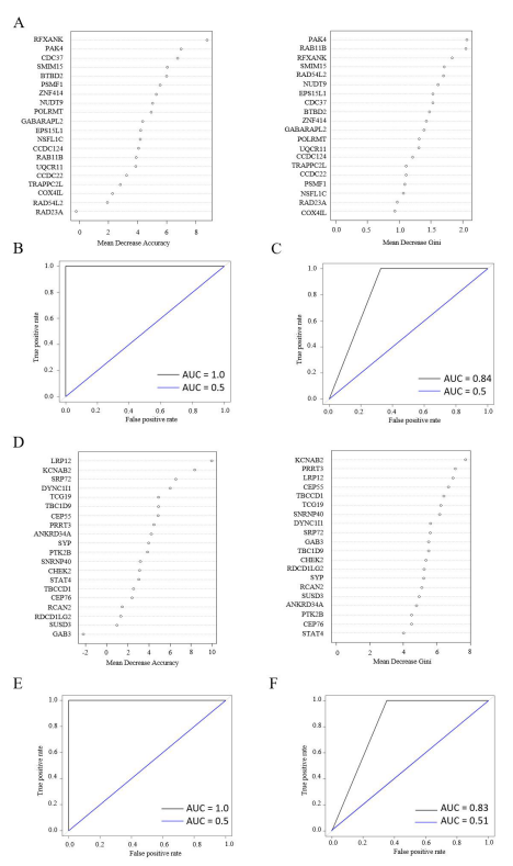
Figure 7: Performance of random forest in GBM and LGG for both training and test sets. (A) The variable importance of the selected genes from GBM, and we evaluated the importance on the metric of mean decrease accuracy and mean decrease gini; (B) The ROC of the random forest on training and test sets for GBM, the ROC for training set was in black, and ROC for the test set was in blue; (C) ROC of the random forest after ROSE on training (black) and test (blue) sets;(D)The variable importance of the selected genes from LGG, and evaluated the importance on the metric of mean decrease accuracy and mean decrease gini; (E) ROC of the random forest on training (black) and test (blue) sets, respectively; (F) ROC of the random forest after ROSE on training (black) and test (blue) sets.

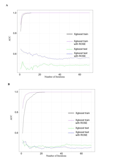
Figure 8: AUCs on Xgboost algorithm in training and test sets before and after ROSE. (A) Using 20 genes in GBM that were selected from elastic net, and put them into Xgboost. The x-axis is the number of iterations and y-asix is the value of AUCs. Each line represents the model performance on that dataset, the black and green curves represent the training and test sets before ROSE, and the purple and blue curves represent the training and test sets after ROSE; (B) In LGG, we applied the 20 genes in LGG selected from elastic net and ran the Xgboost, the performances of each group were shown in the plot.

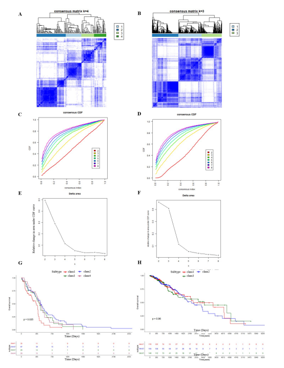
Supplementary Figure 1: Consensus clustering analysis in GBM and LGG. (A) According to the consensus clustering algorithm, the patients in GBM were clustered into 4 groups; (B) and (F) With the plot of CDF under k=2 to 8, we were able to pick the number of cluster between consensus index at 0.1 to 0.9. Ideally we tend to choose the number with the smallest diffrence between the two consensus index cutoff; (C) and (G) Following the CDF plotted in B and F, each point in C and G represents the area under the CDF at particular number of cluster. We usually pick the number after the sudden drop of the area from previous point, and the next k does not change much as the current number. In this case, we picked k=4 and k=3 for GBM and LGG respectively; (D) and (H) The Kaplan Meier curves of each class clustered by the algorithm, with overall survival on the y axis and time by days, whereas only the clusters in GBM showed group differnces (p =0.025).

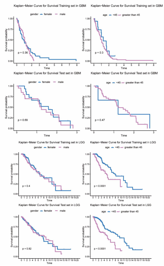
Supplementary Figure 2: Assessment of the diffrence in survival outcome between clinical subtypes in glioma patients. A). Comparison of the survival outcome of the diffrence in gender and age groups in the training and test sets in GBM patients, respectively. Gender and age groups did not show survial diffrence in GBM patients. B). Comparison of the survival outcome of the diffrence in gender and age groups in the training and test sets in LGG patients, respectively. Patients under the age of 45 have a better survival rate than those over 45.

Supplementary Figure 3: Parameters of feature selection using elastic net. (A) The plot showed the changes in accuracy when the algorithm takes in diffrent values of regularization parameter where the blue dotted line represent a series of parameter that was equally cut between 1e-04 to 0.05, the same to all the other lines; (B) The variable importance of the features selected by elastic net after we obtained the optimal value from previous plot;(c) The forest plot of the 20 selected variables and ran them into survival analysis, none of the 20 genes showed survival related (p< 0.05); (D) The plot of the changes in accuracy when the mixing percentage changes at different value of regularization parameters; (E)The top 20 ferroptosis related lncRNAs in LGG that were selected from elastic net, and ranked with variable importance. F). None of the 20 lncRNAs were significantly related to survival.