Figure 1: Workflow Standardized XRD File Processing

Figure 2: Workflow Architecture Design of the Plug-in System

Figure 3: Introduction Diagram Showing the Main Interface UI of oneXRD

Figure 4: Visualization of the phase identification process for CaTiO₃. The experimental peaks (blue stems with 'o' markers), representing data from an unknown sample, are compared against the theoretical diffraction pattern (red dashed stems) calculated from a standard CaTiO₃ CIF file via Bragg's Law. The green “match!” arrow indicates a successful correspondence between the experimental peak position and the theoretical peak position, thereby confirming the identity of the phase.

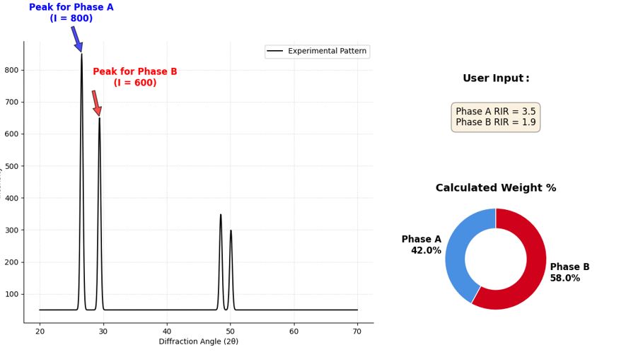
Figure 5: Principle of the Reference Intensity Ratio (RIR) method for quantitative phase analysis, as implemented in oneXRD. The process begins with the user identifying a representative peak for each phase in the experimental diffraction pattern (left panel, e.g., Phase A intensity I=800, Phase B intensity I=600). As shown in the upper right corner, once the user has set the RIR values for A and B, the system will automatically begin calculations and display the results visually, as shown in the pie chart in the lower right corner.

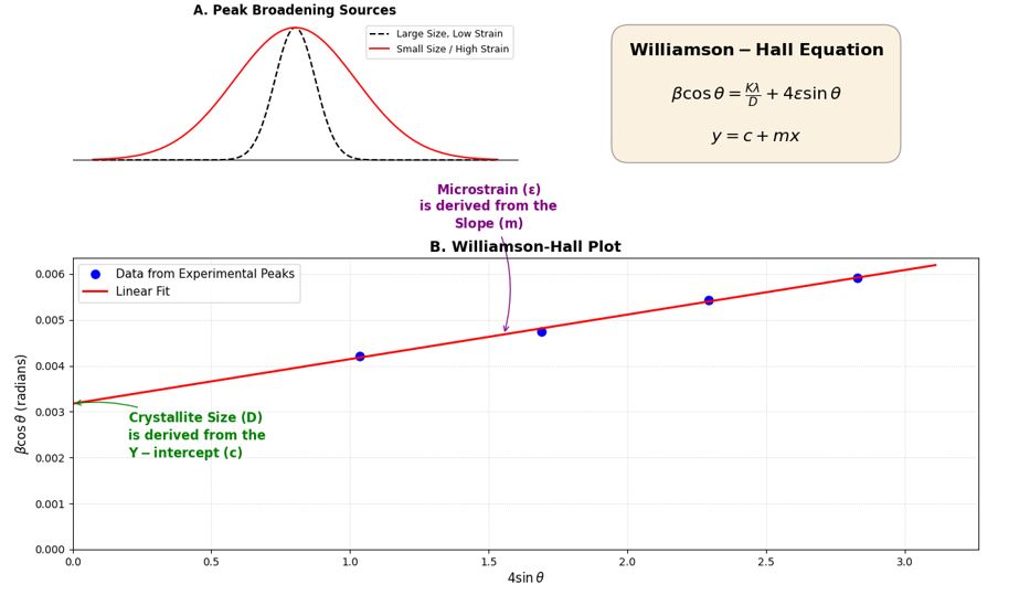
Figure 6: Schematic diagram of Williamson-Hall (W-H) analysis for microstructure determination, implemented in the oneXRD microstructure analysis plugin. (A) The broadening of diffraction peaks is caused by both small grain size and the presence of microstrain. (B) The W-H method separates these two contributions by plotting the transformed peak width data (βcosθ) against the diffraction angle function (4sinθ). The resulting data points are then fitted linearly.

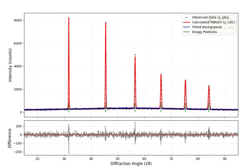
Figure 7: An example figure showing the successful results of Rietveld refinement, generated by the rietveld_refinement plugin in oneXRD. The figure above shows the precise overlap between the experimental data (black dots, y_obs) and the theoretically calculated pattern (red line, y_calc), which is based on a structural model optimized using the least squares method. The fitted background is shown as a blue curve, and the allowed Bragg peak positions are marked with green vertical scales. The figure below shows the difference curve (gray curve), which plots the residual intensity between the experimental and calculated diffraction patterns.

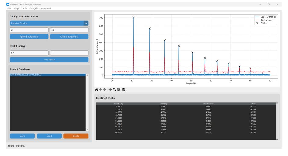
Figure 8: Processed XRD pattern of NIST SRM 660c (LaB₆) in oneXRD. The plot displays the raw experimental data, the calculated background (red dashed line) after iterative erosion, and the automatically identified peaks (black 'x' markers).

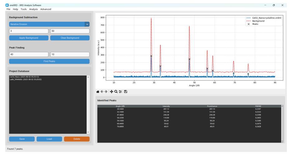
Figure 9: Processed XRD pattern of nanocrystalline CeO₂ in oneXRD. The plot shows the raw data, the subtracted background, and the seven peaks identified for analysis. The significant broadening of the peaks is visually apparent.

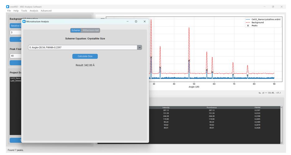
Figure 10: Scherrer analysis result in oneXRD. Using the (111) peak at 28.54° with an FWHM of 0.2397°, the calculated crystallite size is 342.00 Å (or 34.2 nm).

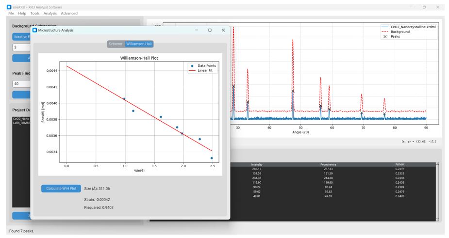
Figure 11: Williamson-Hall analysis result in oneXRD. The W-H plot shows a reasonable linear trend (R-squared = 0.9403). The analysis yields an average crystallite size of 311.06 Å (or 31.1 nm) and a microstrain of -0.00042 (or -0.042%).

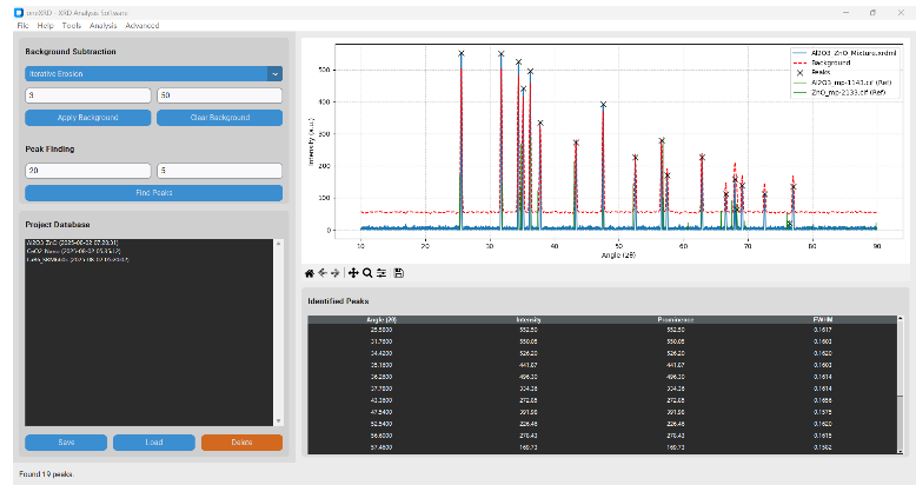
Figure 12: The oneXRD main window showing the fully prepared analysis. The experimental data from the mixture is plotted, the background is subtracted, peaks are found, and the two reference patterns for Al₂O₃ and ZnO are overlaid.

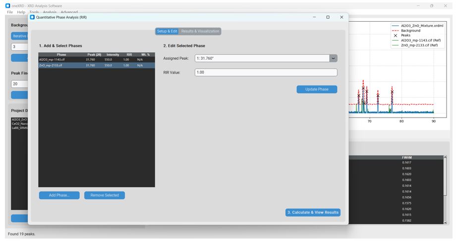
Figure 13: The "Setup & Edit" tab of the QPA plugin. This view demonstrates the seamless workflow where the two phases are preloaded. The user has assigned the appropriate experimental peaks to each phase using the "Inspector" panel.

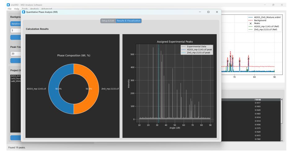
Figure 14: The "Results & Visualization" tab of the QPA plugin. After calculation, the plugin automatically switches to this dashboard, displaying a clear pie chart of the phase composition and a validation plot showing the location of the assigned peaks relative to the full experimental pattern.

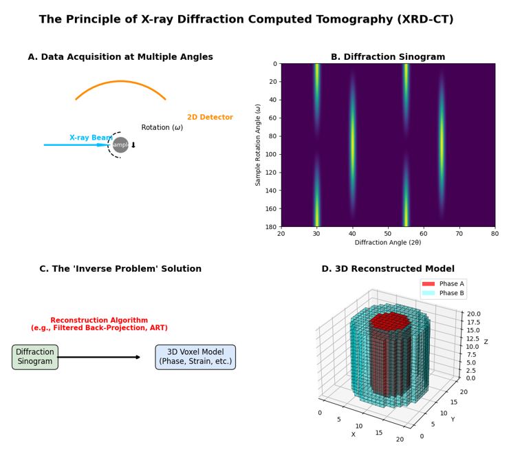
Figure 15: Schematic illustration of the X-ray Diffraction Computed Tomography (XRD-CT) process, the scientific basis for the 3D reconstruction feature in oneXRD.

(A) Data acquisition involves collecting a series of two-dimensional diffraction patterns while the sample is rotated through multiple angles (ω). Unlike medical CT which measures a single absorption value, each projection here contains a full diffraction pattern. (B) The collected data is arranged into a "Diffraction Sinogram," where each row represents a full 1D diffraction pattern (azimuthally integrated from the 2D detector) at a specific rotation angle. The sinusoidal traces indicate the changing orientation of different phases relative to the X-ray beam. (C) A reconstruction algorithm, such as Filtered Back-Projection or ART, is then employed to solve the complex "inverse problem," calculating the most probable diffraction properties for each internal point of the sample. (D) The final output is a 3D voxel model where each voxel contains structural information. This allows for the visualization of the spatial distribution of different phases (e.g., Phase A core in red, Phase B shell in cyan), crystallite orientation, or strain, effectively transforming 2D diffraction "fingerprints" into a 3D structural "body scan" of the material.

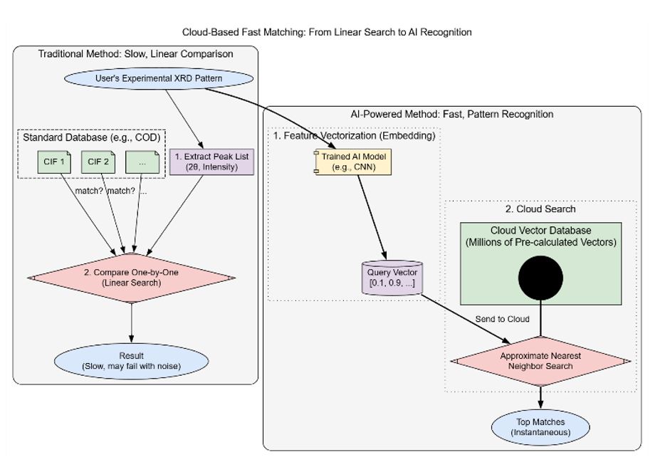
Figure 16: Comparison Flowchart for the Design of the oneXRD Cloud-based Rapid Comparison System

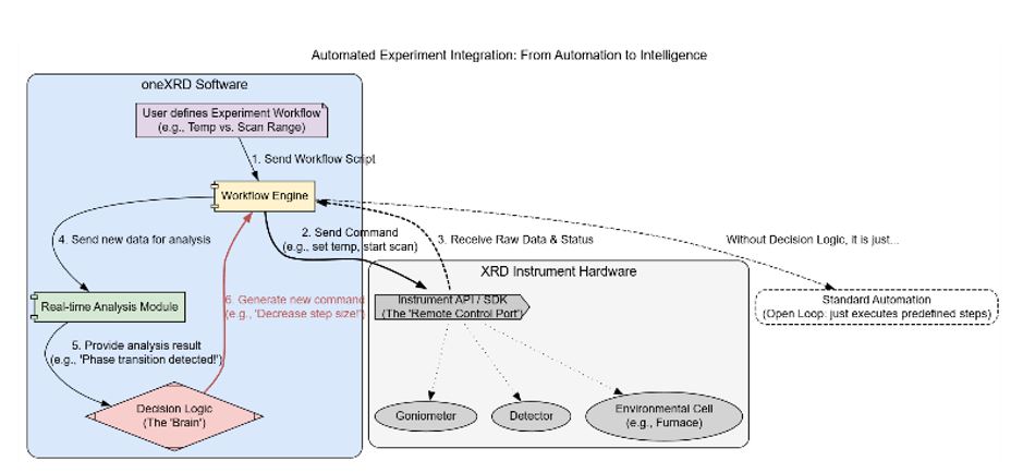
Figure 17: How oneXRD evolved from data analysis software into an experimental control and decision-making center.

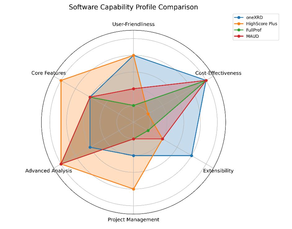
Figure18: A radar chart comparing the software capability profiles of oneXRD, HighScore Plus, FullProf, and MAUD across six key metrics. The diagram illustrates oneXRD's unique strategic position, scoring highly in User-Friendliness, Cost-Effectiveness, and Extensibility—areas where established tools show significant trade-offs. While the commercial HighScore Plus excels in features at a high cost, and the academic FullProf and MAUD offer powerful analysis with a steep learning curve, oneXRD provides a balanced, accessible, and powerful platform for modern XRD analysis.