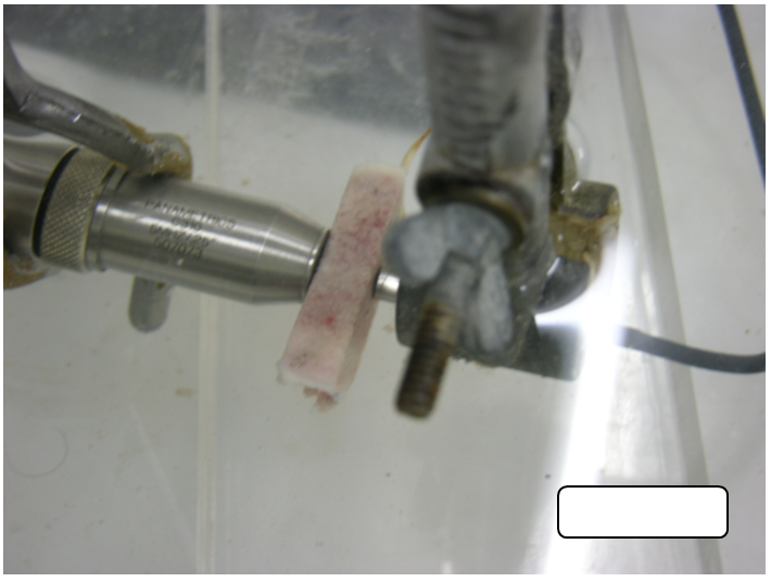
Figure 1: The experimental configuration for a transmission (Tr) mode measurement, with a TB slice between two US transducers - one as Tr the US signal and the other - for its reception (Rec).

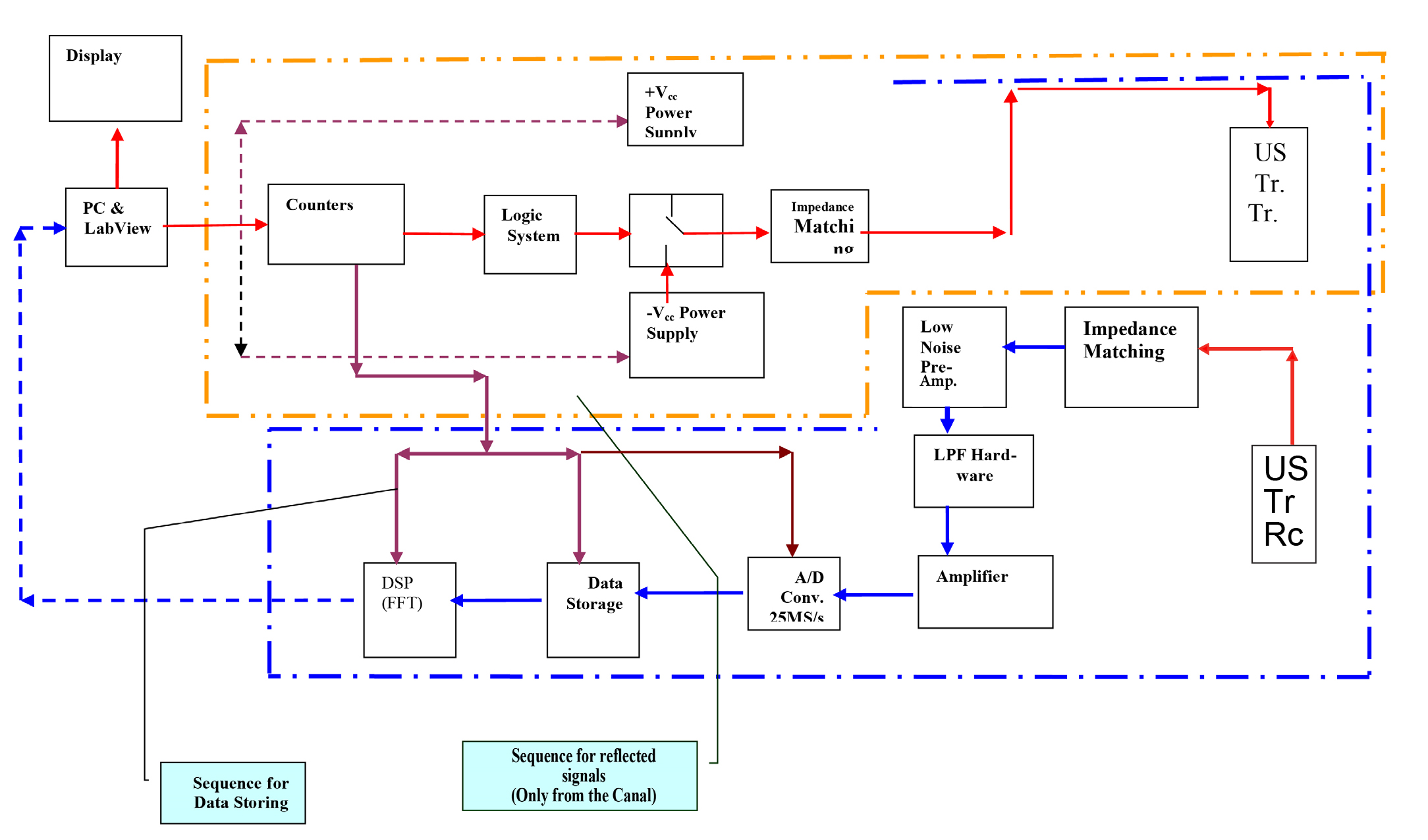
Figure 2: Block Diagram of the Electronic System.

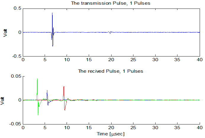
Figure 3: Transmission of 5 MHz, 1 pulse/burst, in the upper plot. In the lower plot, are presented 3 received signals, referring to the 3 slices with different thicknesses: green - slice 1 (4.5 mm), red - slice 2 (14 mm), blue - slice 3 (8.3 mm).
Note:
* It is expected that the received amplitude from slice No.2 (14mm) would be smaller than from slice No.3 (8.3mm) - presumably caused by a slightly different setups of the measuring system (i.e. the TB surfaces where the US transducers are attached, were not smooth enough, thus causing to a loss of energy). This situation repeats with 3 and 6 pulses/burst.

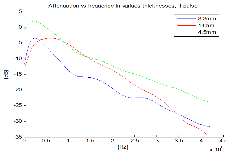
Figure 4: Attenuation vs. frequency fUS = 5 MHz, and Tr of 1 pulse/burst.
Notes:
(i) At higher frequencies the attenuation is higher. The attenuation, in dB, is closely linear with frequency, in the range of ~0.2 106 Hz to ~4.5 106 Hz.
(ii) The attenuation of slice no. 2 (blue) of 8.3 mm, is higher than of slice no. 3 (red)of 14 mm, an anomaly already observed and explained in Figure 3.

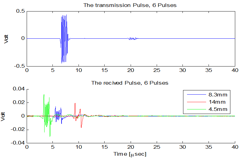
Figure 5: The upper plot described the Tr signal of 6 pulses/burst at fus = 5MHz. The lower plot describes the Rec signals, as they refer to different attenuations in these slices i.e., Blue - slice 1 (8.3 mm), Red slice 2 (14 mm) and Green - slice 3 (4.5 mm).
Note:The red slice (thickness = 14 mm), does not contain in its ReC signal all the 6 pulses; and the Rec signal is completely distorted

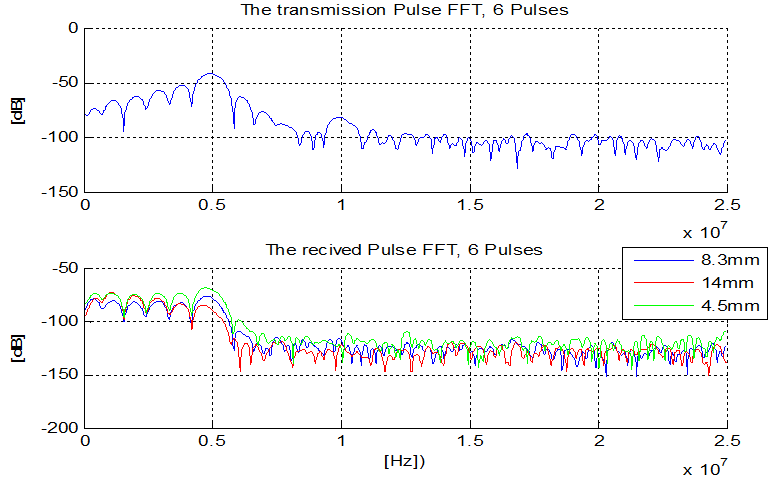
Figure 6: Spectral response of Tr and Rec signals, for fUS = 5 MHz, 6 pulses/burst, for the 3 samples: Blue - slice 1 (8.3 mm), Red - slice 2 (14 mm) and Green - slice 3 (4.5 mm).
Note:
(i) The higher side-lobes (SL) in the Rec spectral response, are highly attenuated, while the main lobe and the lower frequencies SL are attenuated by ~ 25 dB, thus, they are observable and are able to provide carried information.
(ii) The Lower SL are attenuated by ~20 dB, on average.
(iii) The main lobe is attenuated by ~25 dB.

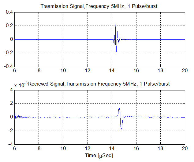
Figure 7: The Tr and Rec signals at 5 MHz, 1 pulse/burst. The Rec signal is broader.

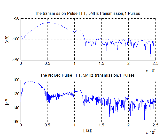
Figure 8: Spectral response of Tr and Rec signals, at 5 MHz, 1 pulse/burst.
Note: Frequencies higher than ~1 MHz are attenuated by 40 to 50 dB; similarly, the main lobe - thus they are submerged in noise and only the LF SL is attenuated by ~20 dB and is well observed.

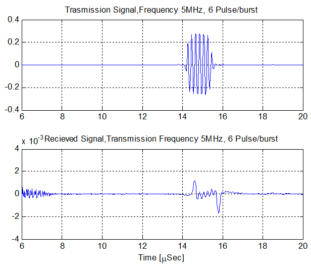
Figure 9: The Tr and Rec signals vs. time, at fUS = 5MHz, 6 pulses/burst. The Rec signal is very distorted.

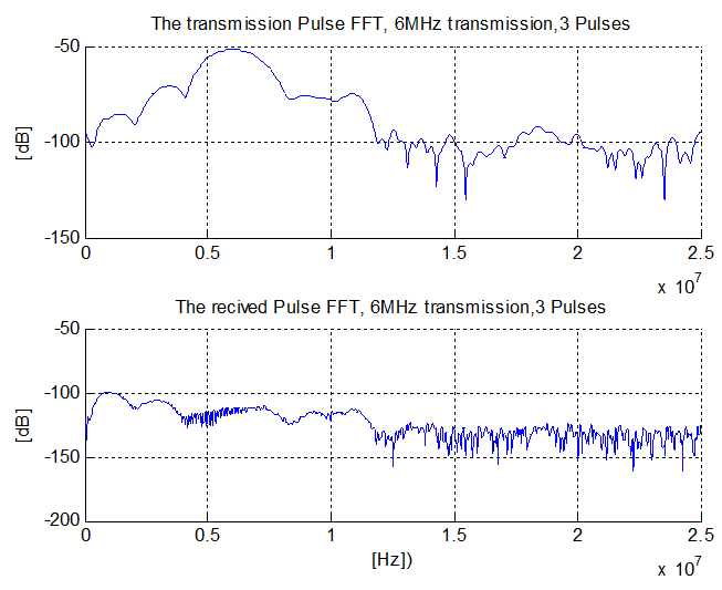
Figure 10: Spectral responses of Tr and Rec signals, at fUS = 6 MHz, 3 pulses/burst.
Note: (i)The high frequency (HF) SL are attenuated more than 75 dB,
(ii)The central frequency (f = 6 MHz) - by 50 dB and
(iii) The LF SL by ~ 25 dB.

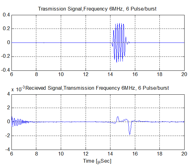
Figure 11: The Tr and Rec signals vs. time, at fUS = 6 MHz, 6 pulses/burst. The Rec signal is very distorted.