Quantitative Finite Element Modelling of Compact Photoacoustic Gas Sensors
Received Date: February 10, 2019 Accepted Date: March 02, 2020 Published Date: March 04, 2020
doi: 10.17303/jmsa.2020.4.101
Citation: Bertrand Parvitte (2020) Quantitative Finite Element Modelling of Compact Photoacoustic Gas Sensors. J Mater sci Appl 3: 1-8.
Abstract
Background: We report on the demonstration of quantitative simulation of compact photoacoustic cells signals. The finite element method is used to calculate the response of differential Helmholtz resonator cells of two different sizes. Simulated quality factors and resonance frequencies are compared with experimental ones. Taking account of the gas sample absorption coefficient and the laser intensity, cell constants are also evaluated and compared to experimental values showing a very good agreement. For compact sensors, where sub-millimeter features are present, the resolution of the pressure acoustics equation is not sufficient to reproduce experimental results and a viscothermal model must be used.
Keywords: Photoacoustic spectroscopy; Gas sensor; Finite Element Modelling; Viscothermal model
Introduction
Laser absorption spectrometry has proved to be a powerful tool for trace gas sensing providing high selectivity of the monitored species and low detection limits. In addition, semiconductor lasers can emit in the mid-infrared region where the fundamental absorption lines of most gases lie. Among laser spectrometry techniques, photoacoustic (PA) spectrometry measures the sound generated in the gas sample cell when exciting the gas with laser radiation [1]. Thanks to resonant cells and differential measurement techniques, PA sensors have shown excellent sensitivities at part-per-billion (ppb) level for most atmospheric gases. These results are comparable to those of other apparatus, such as multipass cells, but with a generally simpler set-up.
The Groupe de Spectrométrie Moléculaire et Atmosphérique of Reims (GSMA, Reims France) has developed since 1997 a photoacoustic sensor with a specific cell design based on Helmholtz resonance [2]. This instrument was originally dedicated to the methane detection with near-infrared diode lasers, then Quantum Cascade Lasers (QCL) appeared as a new opportunity for improvements in gas detection as the PA response is linear with power [3]. More recently the sensor was implemented with a commercial external cavity-QCL emitting at 10.5 μm and allowed the possibility to detect small and complex molecules such as carbon dioxide and butane [4]. For these works, the geometry of the Helmholtz cell was not modified but improvements in the microphone sensitivity and the laser specifications allow decreasing the detection limit down to the ppb level. Detection limits were estimated knowing the cell response, the microphone response, and the gas absorption coefficient at the laser emitting wavenumber. These predictions were then experimentally verified. The cell response was usually compared to simulation using an electric analog circuit method.
In 2006, Baumann et al. proposed to simulate the PA cell responses and resonance frequency using a Finite Element Method (FEM) [5,6]. Our team used the same method to demonstrate for the first time the quantitative modelling of photoacoustic signals including resonance frequency and signal levels quantification [7]. More recently, we also demonstrated the complete optimization and characterization of the sensor for the detection of methane [8] and the possibility to detect methane in large concentrations from 370 ppb up to at least 8% in volume i.e., more than five orders of magnitude with the same Helmholtz sensor [9]. In these papers the experimental results were in very good agreement with the FEM resolution of pressure acoustics equation.
For trace gas measurements, the PA signal is directly proportional to the absorption coefficient of the molecules, to the radiation power and to the cell response. The latter is inversely proportional to the cell volume. This favorable scaling behavior has provoked in recent years a growing interest in the miniaturization of PA cells for gas sensing. The first technique developed to reduce the size of the PA sensors is called Quartz-Enhanced PhotoAcoustic Spectroscopy (QEPAS) [10]. An alternative technique consists in the miniaturization of standard macro-scale PA cells. One can particularly cite the work of Firebaugh [11], later carried on by Pellegrino and Holthoff [12], the realization of 3Dprinted PA cells [13] and the miniaturization of the Helmholtz resonator [14]. However, at the sub-millimeter scale of the chambers and capillaries diameters, the thermal and viscous boundary layers constitute a non-negligible part of the cell volume. Thus, the pressure acoustics description is no more sufficient and a complete viscothermal model taking into account the dissipation effects that must be used to design compact photoacoustic sensors. In this paper, we present the results obtained for devices of various dimensions using two different kinds of FEM simulations based either on the classical pressure acoustics equations or on viscothermal formulation. Both kinds of simulations were performed using a FEM analysis of commercial software [15].
Modelling
Pressure Acoustics Model (PAM)
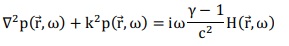
The PAM is commonly used to simulate the PA device behavior. This model is derived from the first principles governing equations, namely the mass, momentum and energy conservation laws supplemented with a thermodynamic equation of state. Assuming adiabatic propagation in an ideal lossless gas and after some manipulation, a single inhomogeneous Helmholtz equation for the unknown pressure is obtained [16]. If harmonic excitation is assumed the equation takes the following form:
where p is the Fourier transform of the acoustic pressure, k = ω/c with c is the sound velocity and ω the angular frequency. Following the reasoning described for instance by Kreuzer [17], and previously used by Baumann et al. [6], it is possible to partly include dissipation effects with the following three steps method:
• determination of the cell eigenmodes, • calculation of coupling between the eigenmodes and the optical excitation, • introduction of dissipation via analytic quality factors corresponding to the various volume and surface loss mechanisms.
Exact solutions exist for simple cell geometries. For more complex geometries, the three steps have to be performed numerically. The PAM and the FEM have been used to describe various PA cells [5-8] and it has been shown that the agreement between FEM simulation and macroscopic PA cell response is good but highly dependent on the accuracy of geometrical representation of the cell in the FEM software. Moreover, when the cell dimensions are of the same order of magnitude than the thicknesses of the viscous and thermal boundary layers, the PAM is expected to be inaccurate and, for microscopic cells, another formulation must be developed.
ThermoAcoustics Model (TAM)
The TAM is especially developed for accurate simulation of acoustics in geometries where some features sizes are in the same order of magnitude as the thermal and viscous boundary layers thicknesses. As the PAM, this viscothermal acoustic model is derived from the mass, momentum, and energy conservation laws supplemented with a thermodynamic equation of state. Small harmonic variations of the variable density, velocity, pressure and temperature fields, are assumed leading to the following set of Partial Derivative Equations (PDEs):
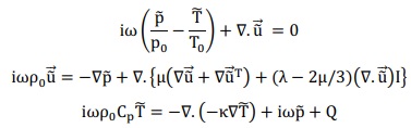
where p~, T~ and u~ are respectively the pressure, temperature and velocity fields in the gas. p0,T0 and ρ0 are the mean values of the pressure, temperature and density fields. l and μ are the bulk and shear viscosity. The bulk viscosity is set to 0.6 μ [18]. κ, Cp and Q are respectively the thermal conductivity, the heat capacity at constant pressure and the volume heat source. I is the identity matrix. The previous PDE system is complemented by a set of boundary conditions. First, at the interface between the cell walls, considered as rigid, and the gas, a no-slip condition is used, imposing a zero gas velocity. Second, as the glass thermal conductivity is much larger than that of the gas, it is assumed that the walls are isothermal, leading to a zero temperature perturbation at the walls.
The set of PDEs and associated boundary conditions are solved by the FEM, using the Thermoacoustics interface of the “Acoustics” module of COMSOL Multiphysics® [15], called the TAM in the rest of the paper. The left part of Figure 1 presents the inner cell volume and an example of mesh. The right part of Figure 1 presents the acoustic pressure repartition of the Helmholtz resonant mode (blue to red color scale) and optical intensity of the laser beam used as excitation (dark red to yellow color scale in the left chamber).
Experimental set-up
PA cells
In [7] we demonstrated for the first time the possibility to quantitatively simulate photoacoustic signals using FEM software and PAM. Quality factors and resonance frequencies were compared with experimental ones demonstrating a very good agreement. We also go further at using the FEM model with PA cells of different shapes [8] and also measurement conditions where the repartition of the laser intensity across PA cell in the FEM model must be taken into account [9], for these studies the method has proved to be robust as well. To explain the remaining differences between FEM and experimental results, some technical characteristics were impossible to precisely determine and
implement in the model such as potential surface defects due to the manufacturing process that are not represented in the perfect 3D geometry of the FEM model, leading to a decrease in the response. Moreover, modeling of PA cells geometry and associated microphones leads to inevitable approximations in terms of shape. In the present study, we especially designed simplified cells permitting to obtain simple shapes and to adapt simple electret microphones (Knowles EK-23133 with a sensitivity of 22 mV/Pa @ 1000 Hz) thus limiting the effect of microphone volumes that are negligible in comparison with the cell volume. A photograph of a cell is given in Figure. 2. This cell is made of glass in order to enhance the surface quality roughness of the resonator walls and thereby limit losses.
Two different cells were designed. The dimensions are given in table 1. Cell #1 has internal dimensions that are chosen to be close to those of [7]. As the original cell was made of cylindrical tubes and that these cells have their main volumes that are square-based, the length of the main volume was adapted in order to keep a volume around 8,000 mm3. The square-based was chosen in order to improve the contact between the microphones and the upper walls of the main volumes, thus limiting dead volumes. Cell #2 was designed to have a homothetic reduction of the dimensions by a factor 4.
Test set-up
Characteristics of the photoacoustic cells are investigated using the setup presented in Figure 3. The laser source is a thermoelectric-cooled continuous-wave Quantum Cascade Laser (cw-QCL) emitting at 1,275.04 cm−1. The laser is operated at 545 mA and 5°C. The QCL is driven by a diode current source (ILX model LDC-3744B) that also regulates the temperature. In front of the laser, a two lenses telescope with 1 mm and 12.3 mm focal lengths is placed to have a ≈1 mm size waist at 75 cm from the laser. A Gaussian beam profile was observed with an infrared camera placed at the cell output. The optical power is measured by a power meter (Ophir model AN/2). A gas dilutor (Alytech Gas Mix) is used to produce different mixtures of methane (Air Liquide, CH4-N55) in dry air (Air Liquide, Alphagaz 1). The dilutor controls the flow rate at the PA cell inlet to maintain a continuous flow during the photoacoustic response acquisition. A mechanical chopper (Thorlabs MC 2000 system) is used to modulate the amplitude of the beam at a given frequency. A lock-in amplifier (E&G model 5301) retrieves signals A, B and |A − B|. A stands for the signal measured at the excited volume, B at the other microphone and |A − B| is the differential measurement. A Lab VIEW program controls the chopper frequency and automatically acquires the resulting PA signal by recording the values from the lock-in amplifier. The room temperature is measured at 20 +/- 2 °C for all the presented data.
The experimental response is investigated by varying the modulation frequency of the chopper from 200 to 2000 Hz with a constant concentration of methane of 1000 ppm at a low flow of 100 mL/min maintain in the cell during the acquisition. This concentration is far higher than the limit of detection of the two cells for methane (typically lower than 10 ppm) thus allowing to obtain very reproducible measurements. Between two frequency steps, a 10-s delay is observed, and the acquisition is made at the end with a lock-in amplifier integration time of 300 ms.
Simulation of Helmholtz cells
For both models, the calculations mainly rely on the physical properties of the gas inside the cell and on the shape of the acoustical resonator. We assume that the cell will be used for the detection of a small amount of absorbing gas diluted in air and use the properties defined for air at T0 = 293 K and P0 = 101,325 Pa in the COMSOL material library. These parameters are presented in Table 2. The absorption coefficient α and the laser power were, respectively, set to 1 cm−1 and 1 W in order to obtain a normalized value Rc in Pa/(W/cm). Note that the physical properties of the cell material are not taken into account in the simulation process and the cell boundaries are considered as perfectly rigid walls.
For each designed cell, the experimental cell parameters (resonance frequency, Q-factor and cell response RC) were measured using the experimental set-up described in section 3.2 and various simulations were performed with COMSOL Multiphysics ® using different kind and refinement of mesh. We use either a standard tetrahedral mesh or an adapted boundary-layer mesh. Nine different predefined mesh qualities were used from 9 (extremely coarse) down to 1 (extremely fine). The maximum and minimum element sizes corresponding to the mesh qualities are summarized in table 3.
Most of the dissipation (viscous dissipation and heat conduction) processes occur in a thin region located near the cell walls. The thickness of this region can be estimated to approximately 0.06 mm for a working frequency around 1 kHz, in air at standard temperature and pressure [6]. Except for the highest mesh quality, this region cannot be correctly described by the tetrahedral mesh (only one element in the boundary region). In order to improve the description of dissipation processes an adapted boundary-layer mesh is used, that refines the mesh near the cell walls and typically adds 4 or 5 meshing elements in the 60 μm region. Total calculation time and memory requirement both increase with the mesh quality and with model complexity. For the simple pressure acoustics model, all mesh qualities were solved whereas for viscothermal acoustic model the highest mesh qualities (2 and 1) computations were not carried out due to memory requirements (Out of memory during LU factorization on a 256 GB workstation).
Cell #1
Calculated resonance frequency, quality factor and cell constant for cell #1 are presented in Figure 4 as a function of the mesh quality and compared to experimental results. The PAM results are less sensitive to mesh quality. The resonance frequency is close to the experimental one (shifted from approximatively 10 Hz, that is a 2.5 % difference). The agreement is very good for quality factor (less than 1 % difference) except for the finest mesh (without explanation). The cell response is clearly more sensitive to mesh quality and for coarser meshes, there may be a factor 2 difference. The value is close to the experimental one only for high-quality meshes. On the contrary, the TAM results are highly dependent on this parameter. As expected, it appears that the TAM using standard tetrahedral mesh (TAM-T) was not adapted even if the TAM with tetrahedral mesh seems to converge towards experimental values when the mesh is refined. Results are closer to the experimental ones when using the boundary-layers mesh (TAM-BL) even if, in this case, the finest mesh qualities cannot be solved, due to memory limitations. The resonance frequency is shifted from 1-2 Hz, i.e. a very good agreement is found for this study. The quality factor agreement is good (10 % difference) and seems to improve when the mesh refines. When using the TAM-BL, both parameters show only a weak dependence on the bulk tetrahedral mesh quality confirming that losses mechanism are mainly located at the boundary layer. The simulated cell response remains close to the experimental one with the TAM. The difference is always lower than 25 % (for the coarsest mesh quality) and diminishes down to approximately 5 % when the mesh refines. The discrepancy between experiment and simulation is greater for cell response than for quality factor. Q This higher discrepancy is probably due to insufficient mesh quality on the path of the laser beam leading to an incorrect value of the absorbed energy. In conclusion, the PAM with the finest mesh gives good results and the TAM with adapted mesh improves the validity of the model.
The TAM-BL simulation results closest to the experimental data are compared with the experimental PA signal for microphones A and B in Figure 5. The agreement is excellent, thus confirming previous results [7] and the possibility to qualitatively simulate the PA signals of macroscopic PA cells, even in case of complex designs. Note that the PAM and TAM differences remain small and we choose to represent only simulations using the TAM-BL on this graph. This excellent agreement is confirmed in Figure 6, where the experimental cell response is compared to simulation results.
Cell #2
Calculated resonance frequency, quality factor and cell constant for cell #2 are presented in Figure 7 as a function of the mesh quality and compared to experimental results. The PAM results are almost insensitive to mesh quality even for the cell response. The resonance frequency is shifted from the experimental one from approx. 100 Hz. The agreement is correct for quality factor (value of compared to 3.4). The cell constant is no more sensitive to mesh quality and the simulated value is overestimated to the experimental one by approximatively 30 %. As for cell #1, the TAM simulations using standard tetrahedral mesh (TAM-T) are not adapted for this simulation. Results are closer to the experimental results when using the boundary-layers mesh (TAM-BL) even if, once again, the finest mesh qualities cannot be used due to memory limitations of the computer. The resonance frequency difference between simulations and experiments is less than 1 Hz, i.e. an excellent agreement. The quality factor agreement is correct (value of 4 compared to 3.4), better than with PAM, and seems to enhance when the mesh is refined. Unfortunately, once again, it was impossible to use finer meshes in order to verify this hypothesis. Finally, as for PAM, the cell response is overestimated, when compared to the experimental one, by approximately 25 %.
In conclusion, for cell #2, the PAM even with the finest mesh does not give sufficiently accurate results. It is necessary to use the TAM with an adapted mesh to obtain the true value of resonance frequency. The other parameters are closer to the experimental values using the TAM than the PAM. The remaining difference for Q-factor and cell response may be observed in detail in Figure 8 where the PAM and the TAM-BL results are compared with the experimental PA signal for microphones A and B. For the PAM signals, the difference in resonance frequency is large and simulation is far from experimental results. The PAM does not accurately describe the characteristics of a centimeter scale cell. Moreover, the PAM does not describe the asymmetry that appears between A and B signals. A stands for the signal measured at the exciting volume and this information is not taken into account in the PAM. On the contrary, the TAM with an adapted mesh (boundary layers) provides an excellent agreement with the experiment for the resonance frequency. Moreover, it describes the asymmetry even if it underestimates it: one can remark than B signal is lower than A signal at maximum as observed in the experimental results. The same observation between models is confirmed in Figure 9 where the experimental cell response is compared to simulation. Both Q factor and cell response are overestimated by the PAM and the TAM, but the TAM gives an excellent value of resonance frequency. In order to understand the origin of discrepancies between experiments and results of the simulation, several studies were performed assuming that the set of equations solved in the TAM accurately describes the sound generation and propagation even in much smaller systems than our cells and that mesh quality in the TAM – BL is sufficient. This assumption seems reasonable since resonance frequency, quality factor and cell constant do not show strong enough dependency on mesh quality to explain the remaining discrepancies. On the opposite, the accuracy of the cell representation in the numerical model seemed to be questionable and several hypotheses were studied:
Deviation from the expected dimensions: The dimensions listed in Table 1 were used both for the mechanical realization and for the numerical model. However, the actual cells may present some deviations from the expected dimensions. In order to study the effect of such deviations, a series of simulations using various combinations of cell dimensions was performed. None of those combinations allowed to reproduce the observed dependences of signals A, B and |A-B| with frequency. The main effects were some shift of resonance frequency, and a variation of Rc. No sensible effect on the asymmetry between A and B was observed. Moreover, the underestimation of A near 1000 Hz was not correctly described.
Localized defect: Due to the fusing process during cells manufacturing, the actual cells may present localized defects like the narrowing of capillaries near the walls (See Figure 2). The effect of such narrowing in one or both capillaries was numerically studied but did not allow to reproduce the observed dependences of signals A, B and |A-B| with frequency: partial obstruction leads to a decrease of Rc associated to a shift of resonance frequency. No sensible effect on the asymmetry between A and B was observed. Moreover, as for the previous case, the underestimation of A near 1000 Hz was not correctly described.
The other kind of difference between the actual cells and the model is due to the acoustics ports for the microphones and to the gas inlet and outlet. Although their dimension remains small compared to the overall cell dimension, the boundary conditions (no-slip condition and isothermal walls) are no longer valid at these points. An accurate description of inlet/outlet and of microphone would have added complexity to the model (additional volumes with Perfectly Matched Layers to represent the tubing for gas inlet/outlet, and elasticity of microphone membrane). We tried to approximate the inlet/outlet and the microphones by adding small circular regions with zero pressure boundary condition located on each capillary (inlet/outlet) and at the microphone's positions. For simplicity, a single radius was used for both inlet and outlet. The same simplification was made for both microphones. Successive trials were performed with various radiuses values in order to better reproduce the experimental data. The main effect of adding inlet/outlet is to modify the cell response near 1 kHz (increase for the A signal and decrease for the B signal). The main effect of adding microphone ports is to decrease A and B at the resonance frequency. The results obtained for 17 μm radius (microphone ports) and 35 μm radius (gas inlet/outlet) are plotted on Figure 8 for A and B signals and on Figure 9 for |A-B| and both show a clear improvement of the agreement with experimental data. These radiuses are much smaller than the actual microphone ports and gas inlet/outlet dimensions but represent the only partial opening of the cell towards the exterior.
Finally, we also verified that the inclusion of circular regions of the same radiuses in the model for cell #1 - that has the same actual microphone ports and gas inlet/outlet dimensions - only have negligible effect: resonance frequency, quality factor and cell constant only vary of a few %. Although this description is not strictly valid due to the use of adjustable parameters, it illustrates the need of stringent accuracy in the conception of the model, especially for small dimensions devices.
Conclusion
In photoacoustic spectroscopy, gas detection limits are usually estimated after the manufacturing and assessments of a photoacoustic cell. Using a Finite Element Method (FEM), our team has previously demonstrated that the quantitative modeling of photoacoustic signals including resonance frequency and signal levels quantification was possible with simulation using a Pressure-Acoustics Model (PAM). This assessment is demonstrated in this paper, where cell #1 characteristics are perfectly simulated using either the PAM or the Thermo-Acoustics Model (TAM). The only condition is to use the finest mesh for the PAM and an adapted (boundary-layers refined) mesh for the TAM.
However, this description is only valid when the size of the cell remains in the tens of centimeters range. For more compact photoacoustic sensors (here cell #2), as expected, it was demonstrated that the PAM is not valid anymore and that the TAM, taking into account the dissipation effects, should be preferred to perfectly describe the resonance frequency. Even in this case both Q factor and cell constant remain slightly overestimated. In order to understand the origin of the remaining discrepancies between experiments and results of the simulation, several studies were performed such as deviations from the expected dimensions or localized defects but without success. Finally, the remaining differences have be explained by the presence of gas inlet/outlet and to the microphone ports. Final simulations including leaks show a very good agreement between experiment and simulations for the three parameters: resonance frequency, quality factor, and cell response.
Acknowledgement:
The authors acknowledge Christophe Risser, Justin Rouxel and Alain Glière for their valuable contribution to this work.
- MW Sigrist (1994) “Air Monitoring by Spectroscopic Techniques”.
- V Zéninari, VA Kapitanov, D Courtois, YN Ponomarev (1999) “Design and characteristics of a differential Helmholtz resonant photoacoustic cell for infrared gas detection”, Infrared Phys. Technol. 40: 1-23.
- A Grossel, V Zéninari, L Joly, B Parvitte, D Courtois, G Durry (2006) “New improvements in methane detection using a Helmholtz resonant photoacoustic laser sensor: a comparison between near-IR diode lasers and mid-IR quantum cascade lasers”, Spectrochim. Acta A 63: 1021-1028.
- D Mammez, C Stoeffler, J Cousin, R Vallon, MH Mammez, L Joly, B Parvitte, et al. (2013) “Photoacoustic gas sensing with a commercial external-cavity quantum cascade laser at 10.5 μm”, Infrared Phys. Technol. 61: 14-19.
- B Baumann, B Kost, H Groninga, M Wolff (2006) “Eigenmode analysis of photoacoustic sensors via finite element method”, Rev. Sci. Instrum. 77: 044901.
- B Baumann, M Wolff, B Kost, H Groninga (2007) “Finite element calculation of photoacoustic signals”, Appl. Opt. 46: 1120-1125.
- B Parvitte, C Risser, R Vallon, V Zeninari (2013) “Quantitative modelization of photoacoustic signal”, Appl. Phys. B 111: 383-389.
- C Risser, B Parvitte, R Vallon, V Zeninari (2015) “Optimization and complete characterization of a photoacoustic gas detector”, Appl. Phys. B 118: 319-326.
- V Zeninari, R Vallon, C Risser, B Parvitte (2016) “Photoacoustic Detection of Methane in Large Concentrations with a Helmholtz Sensor: Simulation and Experimentation”, Int. J. Thermophys 37: 1-11.
- AA Kosterev, YA Bakhirkin, RF Curl, and FK Tittel (2002) “Quartz-enhanced photoacoustic spectroscopy”, Opt. Lett. 27: 1902-1904.
- S Firebaugh, K Jensen and M Schmidt (2002) “Miniaturization and integration of photoacoustic detection”, J. Appl. Phys. 92: 1555-1563.
- EL Holthoff, DA Heaps, and PM Pellegrino (2010) “Development of a mems-scale photoacoustic chemical sensor using a quantum cascade laser”, IEEE Sens. J. 10: 572-577.
- R Bauer, G Stewart, W Johnstone, E Boyd, M Lengden (2014) “3D-printed miniature gas cell for photoacoustic spectroscopy of trace gases”, Opt. Lett. 39: 4796-4799.
- J Rouxel, JG Coutard, S Gidon, O Lartigue, S Nicoletti, B Parvitte, R Vallon, V Zéninari, A Glière (2016) “Miniaturized differential Helmholtz resonators for photoacoustic trace gas detection”, Sensors and Actuators, B: Chemical 236: 1104-1110.
- COMSOL Multiphysics® v. 5.2. www.comsol.com. COMSOL AB, Stockholm, Sweden.
- PM Morse, K Uno Ingard (1968) “Theoretical acoustics” (Princeton University Press).
- LB Kreuzer (1977) “The physics of signal generation and detection,” in Optoacoustic spectroscopy and detection 1–25.
- WM Beltman (1999) “Viscothermal wave propagation including acousto-elastic interaction, part I: Theory”, Journal of sound and vibration 227: 555-586.
FIGURE 1
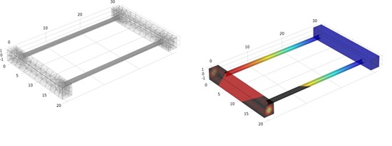
Figure 1: Mesh of the cell volume (on the left) and repartition of the first calculated mode (on the right) for a standard Helmholtz resonator. In this Helmholtz resonance, both signals are opposite in phase. A differential measurement aims to subtract environmental noises as the signal of interest is doubled. The intensity repartition of the laser beam is also represented in the left chamber of the cell.
FIGURE 2
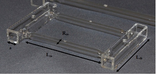
Figure 2: Photograph of the compact glass cell #2 especially designed for this study.
FIGURE 3
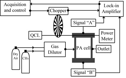
Figure 3: Block diagram of the experimental setup
FIGURE 4
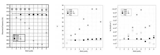
Figure 4: Resonance frequency, Q-factor and cell #1 response in function of the mesh quality ("1" = Extremely fine and "9" = Extremely coarse)
FIGURE 5
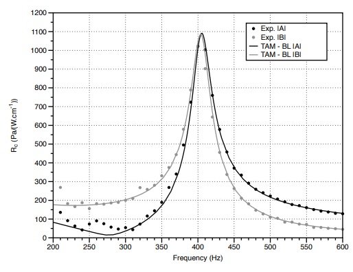
Figure 5: Microphones A and B responses for cell #1 in the function of the excitation frequency. Experimental data are represented by dots whereas modeling results are in solid line.
FIGURE 6
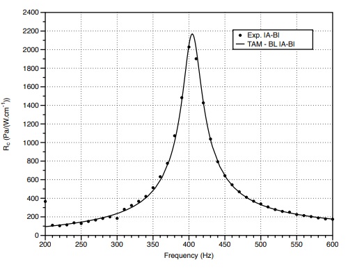
Figure 6: Cell #1 response in function of the excitation frequency.Experimental data are represented by dots whereas modeling results are in solid line.
FIGURE 7
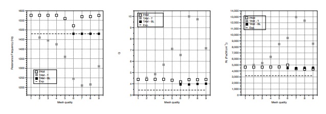
Figure 7: Resonance frequency, Q-factor and cell #2 response in function of the mesh quality ("1" = Extremely fine and "9" = Extremely coarse)
FIGURE 8
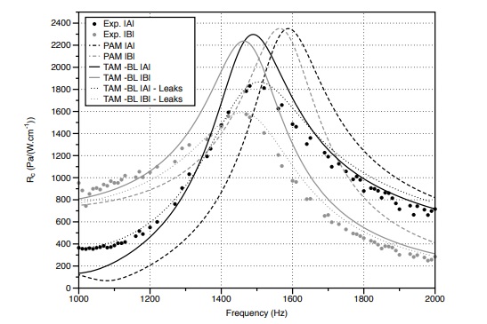
Figure 8: Microphones A and B responses for cell #2 in function of the excitation frequency. Experimental data are represented by dots whereas modeling results are in dashed line for PAM, in solid line for TAM-BL and in dotted line for TAM-BL with model including leaks.
FIGURE 9
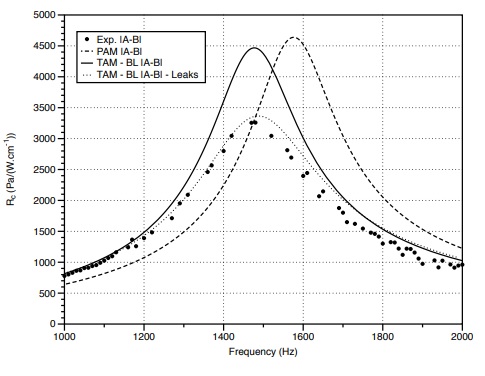
Figure 9: Cell #2 response in function of the excitation frequency.Experimental data are represented by dots whereas modeling results are in dashed line for PAM, in solid line for TAM-BL and in dotted line for TAM-BL with a model including leaks.
Tables at a glance
Figures at a glance