Tables at a glance

Table 1

Table 2

Table 3

Figures at a glance

Figure 1

Figure 2

Figure 3

Figure 4

Figure 5

Figure 6

Figure 7

Figure 8

Figure 9

Figure 10

Figure 11

Figure 12

Figure 13

Figure 14

Figure 15

Table 1

Parameter	DT
y	335
C_dMJ.g^-1(g/c³s)^2/3	0 32
a
M(mg)	1.24

Table 1: Numerical values of different parameters for calculation energy gain

Table 2

pR2	pRl	f r	Gmax DT
2. 184	<0.852	0.0500	284.33
2. 379	<0.780	0.0792	310.64
2. 617	0.733	0.1083	329.86
2. 823	0.703	0.1375	344.29
2. 970	0.682	0.1667	355.24
3.072	0.667	0.1958	363.49
3.146	0.655	0.225	369.57
3.195	0.648	0.2542	373.79
3.225	0.643	0.2833	376.38
3.238	0.641	0.3125	380.79

Table 3

	Beam number	Energy per beam	duration
ps lasers	8	2.5 kJ/10 ps/1w	1 - lops
ns lasers	32	8KJ/10ns/1w	0.2 - 20 ns

Table 3: The proposed laser parameters for DCI design which is used here

FIGURE 1

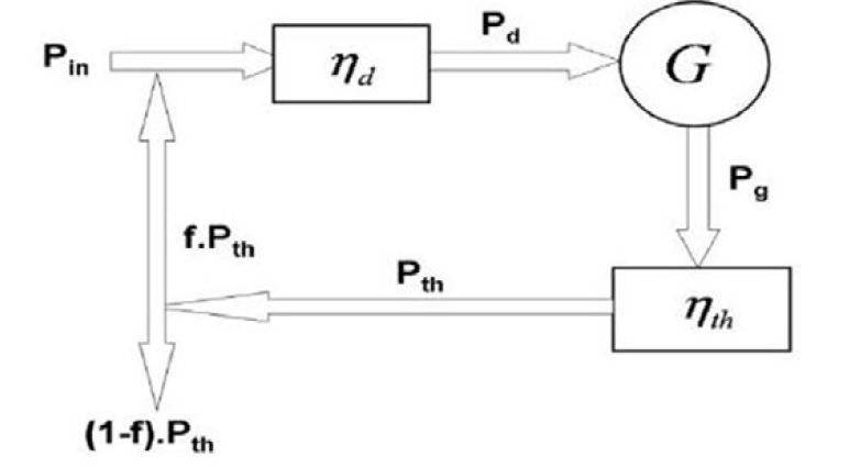
Figure 1: Power cycle.P_in , the input power (this could be the electrical power from the outlet).P_d , the power at the output of the driver.P_g , the power from thermonuclear fusion

FIGURE 2

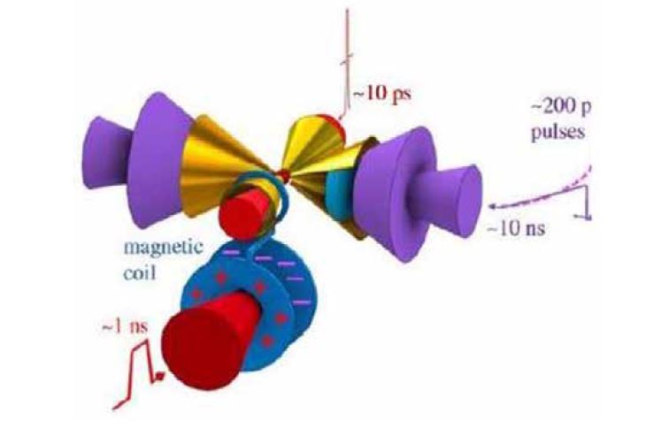
Figure 2: Schematic of the DCI. The fuel is initially installed at the inlet of the two main cones in horizontal directions. Two processes of acceleration and compression are performed on the main cones. Between the cones, a vacuum space of approximately 100 micrometers is embedded for the collision process. An additional pair of cones can be placed on the vertical plate to conduct laser pulses of ps, PW and produce hot electron beams. If a magnetic field ignition design is adopted, only two additional cones are taken along the direction of the magnetic field. [10]

FIGURE 3

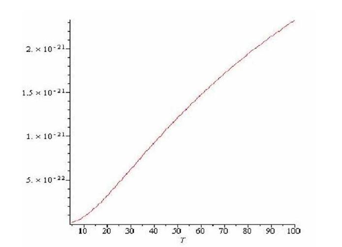
Figure 3: Variations of in terms of temperature

FIGURE 4

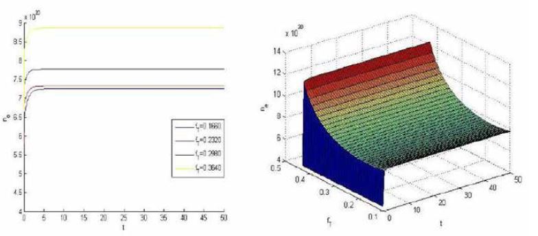
Figure 4: a:Two and b:three dimensional variation of plasma density in terms of time for different values of f_T

FIGURE 5

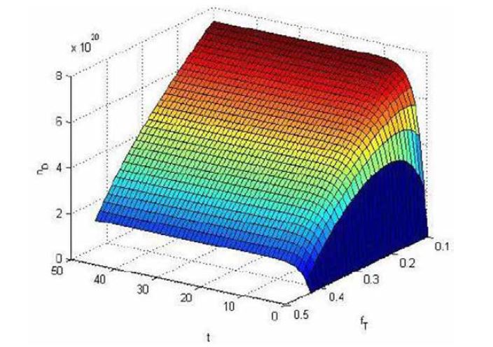
Figure 5: Three dimensional variations of deuterium density versus time and f_T

FIGURE 6

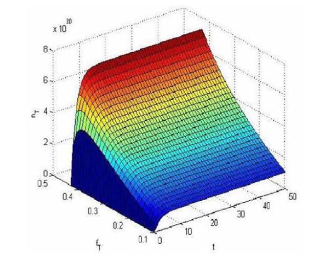
Figure 6: The three dimensional variations of tritium density versus time and f_T

FIGURE 7

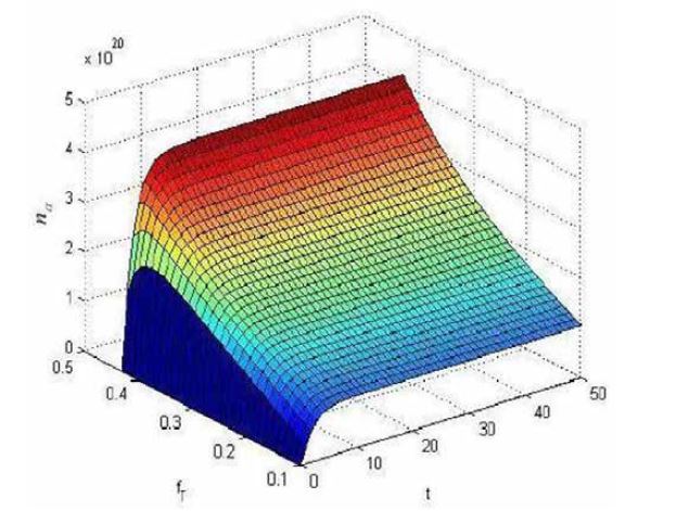
Figure 7: The three dimensional variations of alpha particle density versus time and f_T

FIGURE 8

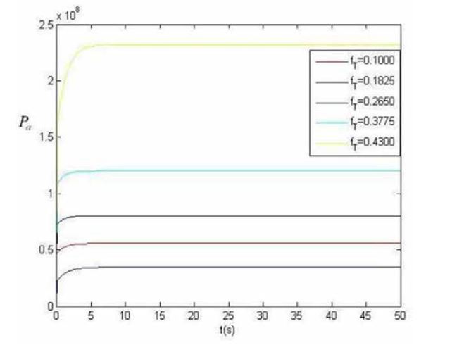
Figure 8: Two dimensional variations of P_α versus time for several values of f_T

FIGURE 9

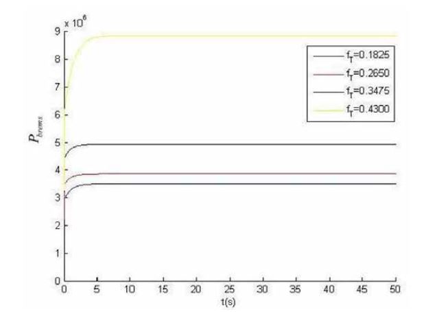
Figure 9: Two dimensional variations of P_berms versus time for several values of f_T

FIGURE 10

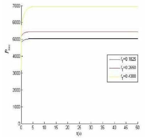
Figure 10: Two dimensional variations of P_loss versus time for several values of f_T

FIGURE 11

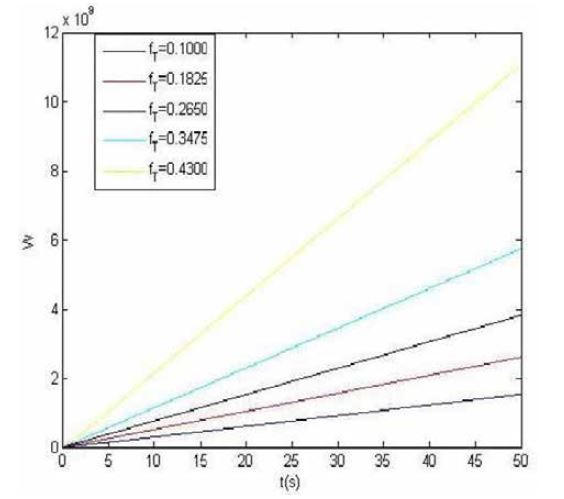
Figure 11: Variations of energy density in terms of time for several f_T

FIGURE 12

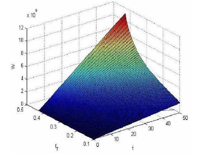
Figure 12: Three dimensional variations of energy density in terms of time and f_T

FIGURE 13

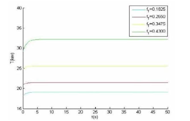
Figure 13: Variations of T_i (ionic temperature) versus time for different values of f_T . From this figure we see that , for each value of f_T by raising time T_i is increased to a maximum value and then becomes constant because by increasing time system achieve a steady state and by increasing f_T the number of fusion reactions are increased therefore more energy is released and temperature of system is increased.

FIGURE 14

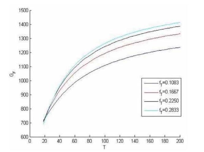
Figure 14: Variations of energy gain versus temperature for different values of f_T at ρR =1.2

FIGURE 15

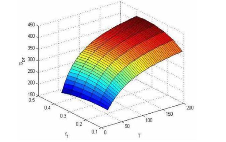
Figure 15: The three dimensional variations of total energy gain in terms of f_Tand temperature at