Energy-Efficient Wavelet Image Fusion Technique in Wireless Sensor Networks for Internet of Things Applications
Received Date: February 16, 2022 Accepted Date: February 17, 2022 Published Date: March 16, 2022
doi: 10.17303/jnsm.2022.8.101
Citation: Mohsen Nasri, (2022) Energy-Efficient Wavelet Image Fusion Technique in Wireless Sensor Networks for Internet of Things Applications. J Nanotech Smart Mater 8: 1-22
Abstract
The Internet of Things (IoT) is a concept in which billions of intelligent devices are connected together. In the IoT systems, smart devices can interact and communicate with one another and with the environment by transferring data and information sensed about the surroundings. Under this concept, multiple sensors are dynamically connected to the internet allowing them to share information in semantically interoperable ways all over the world. Therefore, massive amounts of data are generated and sent over the network. As a result, these applications necessitate a lot of storage, a lot of computing power to enable real-time processing, and a speed network. In this paper, we present an energy-efficient data fusion and processing approach aiming to reduce the size of data collected and transmitted over the network while maintaining data integrity. This method is designed for sensors that have limited energy and processing resources. Our proposed technique is composed of two stages: on-data fusion and in-data compression method. The first stage uses the clustering technique to fuse the sensed data. The second stage uses the wavelet image transform to reduce the amount of processed data and therefore would facilitate a progressive image’s transmission. The paper focuses on the suggested method’s design, modeling, and simulation using the VHDL programming language. In terms of memory and time factors, the design will be compared to existing approaches, and the speed and existing hardware will be optimized. Xilinx 14.2 ISE software was used to create the design, which was then synthesized on a Virtex4 XC4VSX35 FPGA.
Keywords: Internet of Things, Wireless Sensor Networks, Image fusion, Discrete Wavelet Transform (DWT), Field Programmable Gate Array (FPGA)
Introduction
In the recent years, the number of smart connected devices is rapidly expanding, all of which collect and share data in IoT-based systems. Several advanced IoT applications, such as intelligent healthcare systems, smart transportation systems, smart energy systems, and smart buildings, are enabled by the recent advancement [1]. The unified architecture of IoT networks includes smart IoT-based application services as well as the underlying IoT sensor networks. According to Gartner, the IoT global market is expected to reach 5.8 billion IoT-based applications by 2020, up 21% from 2019. From another estimate [2], there will be 80 billion smart items in 2025, with 9.8 linked gadgets per person.
Wireless sensor networks (WSNs) are an essential element of IoT technology since they allow heterogeneous systems, data, and applications to be combined. Sensor nodes in such systems are capable of sensing the required data, performing some processing, and interacting with other network nodes. The basic architecture for IoT sensor data processing, data fusion, and data analysis is shown in Fig. 1. Data fusion is one of the processes carried out by sensors nodes.
When using IoT-based WSN for real-time image fusion, some critical points should be considered. Limited computational power, storage capacity, narrow bandwidth, and required energy are some of these challenges. Therefore, an energy-efficient data fusion approach for image transmission in IoT-assisted WSN is taken into consideration. The wavelet image transform is used in this scheme to ensure significant computational and energy savings, as well as communication with low image quality degradation. The proposed scheme is based on a clustering method. The clustering method is a multi-source single-Base station case. Data fusion is accomplished at the Cluster Head (CH) of each cluster, which has several source nodes and one Cluster Head (CH). At the CH, the data perceived by each source node is fused using a specific data processing method [3]. The fused data is then sent to the BS by each CH.
In a wide range of applications, data fusion from numerous sensors is necessary to improve accuracy. It can be used to track a target in a military or surveillance system, monitor the exact location of an on-road vehicle, locate an impediment in the veins of the human body, and so on. The following are some examples of data fusion applications in various domains [4]:
• The multi-sensor data fusion approach can be used in ships, aircraft, factories, and other applications. Data from electromagnetic signals, acoustic signals, temperature sensors, X-rays, and other sources can be combined in these systems for validation and greater accuracy. This integration will improve accuracy and develop trust in the system, which will help in real time maintenance, system failure detection, and remote rectification, among other things.
• Medical diagnosis is a vital system that incorporates the human body and is used to identify disorders such as tumors, lung or kidney abnormalities, internal ailments, and more, using NMR, chemical or biological sensors, X-rays, and infrared imaging, among other methods.
• Many satellites, aircraft, and subterranean or underwater equipment use seismic, EM radiation, chemical, or biological sensors to collect precise data or identify natural events in long-distance environmental monitoring.
• EM radiation from great distances is used in maritime surveillance, air-to-air or ground-to-air defense, battlefield intelligence, data acquisition, warning, defense systems, and other military and defense applications.
Image fusion has recently gained popularity in these applications because it produces an image that is more valuable in terms of content. Image fusion can be done at three different levels of image data: pixel level, feature level, and decision level [5]. To obtain the fused image, several mathematical computations are done at the pixel level on the intensity values of pixels in the source image. At the feature level, features such as shape, edge, contrast, color, and texture are retrieved from the source images before fusion with the appropriate fusion rule. image. The decision level fusion uses symbolic representations of pictures for the image fusion. These three stages of fusion can be applied to an image’s spatial representation or its transform representation. The multi-scale representation of an image is primarily represented using the pyramid and wavelet representations.
This paper proposes a new energy efficient image fusion based on Discrete Wavelet Transform (DWT). The efficacy of the newly proposed fusion rule is demonstrated in real time on an FPGA board. The EHPF and SHPS approaches are used in this strategy [6]. The 2D-DWT architecture, which is based on the CDF 9/7 standards, as well as the SHPS and EHPF techniques, are discussed in this paper. We developed these architectures using the VHDL programming language. On the FPGA Virtex4 XC4VSX35 platform, we compare the proposed architectures to the conventional architecture in terms of hardware resources, operating frequency, memory capacity, and power consumption.
The rest of the paper is organized as follows: The required background and related work are presented in Section 2. Section 3 presents the Discrete Wavelet Transform. In section 4, the description of the image fusion-based DWT is explained in detail. In section 5, the description of the system model, the data fusion process as well as the data compress center and the data analysis are explained. In the next section, we describe the Implementation and performance analysis and evaluate the output performance; the final part is related to the conclusion and future works.
Related work
In recent years, data fusion has a massive effect in a variety of IoT signal and image processing applications. The data fusion provides several benefits for data processing and analytics, by boosting dataset quality and minimizing data transmission traffic [7]. Due to the large amount of data generated in IoT, data fusion is a difficult task, which increases to the complexity and even introduces inconsistency and conflict data. The data fusion-based energy efficiency systems are used in a wide range of WSN-IoT applications. As depicted in Fig.2, data fusion strategies related to WSN-assisted IoT applications is classified into two categories: (i) Data fusion level, (ii) Data fusion technique.
Multi-sensor fusion, appliance features fusion, and semantic data fusion are the three main application levels of data fusion in the energy efficiency literature. Appliance identification and non-intrusive load monitoring (NILM) are two significant applications of data fusion strategies. Since the power consumption of each electrical device can be derived from the aggregated energy consumption record without the requirement to install a sensor for each application, this application offers interesting insights [8]. Therefore, the cost of implementing energy-saving ecosystems is significantly reduced. Furthermore, several feature fusion techniques can be used to obtain appliance fingerprints, hence boosting the accuracy of appliance recognition. In [9], the authors have proposed a non-intrusive appliance recognition system that provides specific consumption footprints for each equipment. The following steps are used to recognize electrical devices: (a) investigating the applicability as well as performance comparability of several time-domain (TD) feature extraction schemes; (b) exploring their complementary features; and (c) employing a new design of the ensemble bagging tree (EBT) classifier. As a result, a powerful feature extraction technique based on the fusion of TD feature (FTDF) is suggested, with the goal of increasing feature discrimination and optimizing the identification task.
In [10], a multi-sensor fusion technique is proposed. In this case, after the event detection step, appliance features gathered from various domestic devices are fused before applying various unsupervised ML techniques. Multi-sensor fusion aims to reduce probable sensing mistakes by connecting data collected by energy consumption submeters, light, and audio sensors.
Building occupancy detection helps in the reduction of wasted energy and the customization of comfort control. The approach’s goal in [11] is integrated into this framework. authors describe a multi-sensor fusion technique that uses an adaptive neuro-fuzzy inference system (ANFIS) to identify occupancy in a home building. This system monitors ambient circumstances, indoor events, and power consumption patterns from a domestic household, to collect occupancy footprints.
The fusion of high-level information, which is frequently related to decision generation, is referred to as semantic level fusion. Wun et al. propose a high-level semantic data fusion technique that occurs across distinct sensor networks while also aggregating data inside each network in [12]. A semantic data fusion architecture that helps in the aggregation, enrichment, management, and querying data from diverse sensor modalities is proposed in [13].
More recently, complementary research initiatives related to common information fusion techniques for improved performance of IoT applications have been presented. Various methods related to data association were studied in order to enhance the network performance. These methods provide data fusion schemes that rely on the correlation of at least two or more data sources. In [14], the authors propose a new heterogeneous sensors data fusion method for binary occupancy detection, which determines whether or not a location is occupied. This strategy is based on neutrosophic sets and data correlations from sensors.
The state estimation is also a crucial step in the data fusion process. The purpose of state estimation studies is to achieve high state estimation accuracy by combining data from several sensors in various modalities. Maximum likelihood estimation (MLE) [15], Kalman filter [16], particle filter [17], and covariance consistency model [18] are examples of practical approaches related to this class.
The approach of clustering data into distinct categories based on their distinctive properties is referred to as classification. In [19], the authors presented an on-line learning, data-fusion based methodology for increasing temporal resolution of building sensor data using Artificial Neural Networks (ANNs). The proposed method uses sensor data from several sensors around the building to forecast better temporal resolution data from specific sensors.
Methods belonging to prediction class are mainly utilized to predict outputs based on single or multiple information sources. [20] provides an example of some frameworks that use data fusion based on prediction.
The category of unsupervised machine learning relates to fusion systems that try to automate knowledge discovery without the use of ground-truth labels. A structural health monitoring (SHM) system based on the use of a piezoelectric (PZT) active system is introduced for data collecting and management [21]. The proposed technique employs a novelty sensor data fusion for data organization, as well as featured vectors and k-nearest neighbor’s machines, to detect and classify various types of damage.
The statistical inference approaches are used to highlight some distinct traits as well as some common hypotheses retrieved from energy monitoring devices. Two of the most common applications for such techniques are energy disaggregation and appliance identification. The literature contains a large number of papers based on these techniques, such as [22]. In [22], the authors present a methodology based on Integrated Nested Laplace Approximation to predict the energy performance of existing residential building stocks. Five characteristics were identified as possibly significant to assess the building energy performance: urban block pattern, street height-width ratio, building class through the building shape factor, year of construction, and solar orientation of the main façade.
On the basis of relevant platforms, techniques for presenting energy consumption statistics of buildings and their appliances have been implemented [23]. Multiple data sources are fused to create a powerful energy consumption visualization tool that provides end-users with relevant information about the elements that affect their energy usage.
Various methods for energy-efficient data fusion were studied from the above literature in order to enhance the network performance. In order to improve network performance, many strategies for data fusion were investigated from the above literature. Some approaches to data fusion, particularly image fusion in WSN-assisted IoT applications, are not always energy efficient. In this paper, we introduce an energy-efficient image fusion Technique novel which is suitable for resource-constrained Wireless Internet-of-Thing’s Sensor Networks Application. This method is based on DWT and topology clustering.
The Discrete Wavelet Transform
The wavelet transform has lately acquired popularity in signal fusion research in general and image fusion in particular. Wavelet-based coding is more robust under progressive transmission, and also makes image fusion easier. Wavelet fusion methods are particularly well suited to applications where scalability is a very important point to be considered and image degradation may be acceptable. Theoretically, the discrete wavelet transform (DWT) is a two-dimensional separable filtering operation across rows and columns of input image. As depicted in Fig.3, the DWT is based on the concept of multi-resolutions, which reduces the amount of processed data and hence maintains the sensor node restrictions.
A low-pass filter (LPF) is applied to each pixel, followed by a high-pass filter (HPF), line by line and then column by column, to achieve the DWT. We obtain four sub-bands as a result of this process: low-low (LL1), low-high (LH1), high-low (HL1), and high-high (HH1). The original image is down sampled in the low-pass sub-band. The high-pass sub-band represents the original image’s residual information, which is required for a flawless reconstruction of the original set from the low-resolution version. The LL1 sub-band, in particular, can be transformed into the LL2, LH2, HL2, and HH2 sub-bands, yielding a two-level wavelet transform. The third level transform is based on the information provided LL2. Since they reflect the horizontal, vertical, and diagonal residual information of the original image, we refer to the sub-band LLi as a low-resolution sub-band and the high-pass sub-bands LHi, HLi, HHi as horizontal, vertical, and diagonal sub-bands, respectively.
Lifting based DWT
To reduce arithmetic operations as well as the required amount of memory for storage, we based our approach on lifting strategy. Using the lifting-based wavelet transform, the LPF and HPF are broken up into a group of small filters. In comparison to the convolution-based DWT, the lifting approach uses less computations. Therefore, for the DWT implementation in the JPEG2000 standard, a lifting mechanism has been suggested. As shown in Fig. 4, the lifting-based wavelet transform consists of three steps: split, lifting, and scaling.
Where;
a=-1.586134342, b=-0.0529801185, c=0.882911076, d=-0.443506852, and K=1.149604398
The lifting scheme’s basic idea is to first compute a simple wavelet by splitting the original signal into odd and even indexed subsequences, then adjust these values using alternating prediction and updating stages. Following is a description of the lifting scheme algorithm:
• plit step: the original signal is divided into odd and even samples. • Lifting step: this step is divided into N sub-steps depending on the type of filter. Odd and even samples are separated by the prediction and update filters. •Scaling step: After N lifting steps, the lowpass sub-band (YL(i)) and high-pass sub-band (YH(i)) are obtained by applying scaling factors K and 1/K to the odd and even samples, respectively (YH).
Fig. 5. shows how these processes can be used to implement the lifting technique. The lifting strategy for the Daubechies (9, 7) biorthogonal filter used in the JPEG2000 standard for lossy compression is presented in the diagram [24].
The wavelet transform based SHPS technique
The SHPS technique is based on the idea of eliminating the computation of high-pass coefficients [25]. By skipping the least significant sub-band, this technique attempts to save more energy. As a result, the proposal cuts down on arithmetic operations and memory accesses. “SHPS: skipped high pass sub-bands” is the name of the suggested method. High-pass filtering is not used. Therefore, image has a low pass spectrum. As a result, high-pass coefficients were not computed, resulting in the smallest potential loss of image quality. As shown in Fig. 6, the SHPS technique is achieved by making particular adjustments to the wavelet transform.
Using the SHPS technique, the horizontally decomposed low-pass sub-band (L1) is further decomposed in the vertical direction, yielding the LL1 and HL1 sub-bands. During vertical decomposition, the H1 high-pass sub-band is not used. The LL1, HL1, and H1 sub-bands are then produced by the first SHPS level. The image is then processed by applying the 2-D sub-band decomposition to the LLi sub-band and skipping the high-pass sub-band (Hi) in the vertical direction after one transform level. This procedure can be repeated until the desired level is reached.
The wavelet transform based EHPF technique
The proposed image decomposition using the EHPF technique is nearly identical to the SHPS implementation. Using only Low-Pass Filtering following a horizontal decomposition, The LL1 and LH1 sub-bands are maintained, while the HL1 and HH1 sub-bands are removed in this method. Therefore, numerous arithmetic operations will be avoided. The EHPF Multilevel Decomposition approach is depicted in Fig. 7.
The proposed hardware architecture
The proposed architecture is based on the Daubechies (9, 7) filter, which is widely utilized in JPEG2000. This architecture improves the 2D-DWT implementation by making effective use of hardware resources. It is made up of two functional units. The data path unit for data processing and the controller to manage the numerous tasks on the data path. The proposed architecture represents the 2D-DWT algorithm’s line-column mode. After the CDF 9/7 DWT computing in the horizontal direction, a storage stage is required. However, to accelerate the write/read of data, we have opted for using an internal buffer.
Fig. 8 depicts the suggested hardware architecture. It calculates the 2D-DWT in a row-column fashion, on the input image. Each row of the external memory image data’s DWT is calculated by the row filter. Then, the resulting decomposed low-pass and high-pass coefficients are stored in intermediate internal buffers. As soon as the row filter generates enough coefficients, the column filter calculates the vertical DWT of data_L and data_H rspectively. The architecture framework is composed of the following parts: One Line-DWT block, internal buffers, two column-DWT blocks, FiFo_band used for multilevel decomposition, Address generator block and Controller block.
In the beginning of the transform, the input to the 1D-DWT block is the YCrCb component stored in the input memory. A YCrCb component’s pixel is approximately 8 or 9 bits. The filter (9, 7) is called “irreversible” because it is defined using irrational numbers. In general, reversibility cannot be guaranteed in a finite precision floating-point architecture. Therefore, the (9, 7) filter is only suited for lossy compression.
The proposed SHPS architecture
The proposed hardware architecture of the SHPS technique is shown in Fig. 9. The decomposed low-pass coefficients generated after the line-DWT are stored in intermediate buffers and the column filter calculates the column-DWT as soon as there are sufficient coefficients generated by the row filter. On the other hand, the high-pass coefficients, are saved in the FiFo band. Then, the first SHPS level results the LL1, HL1, and H1 sub-bands. Therefore, the proposed SHPS architecture reduces the hardware complexity and memory accesses.
The proposed EHPF architecture
The proposed EHPF-based architecture is similar to the SHPS implementation. As depicted in Fig.10, Only the LL1 and LH1 sub-bands are preserved in the proposed architecture, whereas the two other high-pass sub-bands (HL1 and HH1) are removed. In each decomposition level, the LPF is just used in the column-DWT. One line-DWT block, internal buffers, one column-DWT, LL FIFO used for multilevel decomposition, Address generator block, and Controller block make up the architecture framework.
1D-DWT architecture
A 1-D filter bank transforms the input signals on line-DWT into High (H) and Low (L) component signals. According to the lifting strategy utilizing the filter (9, 7) shown in Fig.6, there are four lifting stages necessary to identify the high and low pass coefficients. As a result, each lifting step of the filter (9,7) can be allocated to a computing module, as shown in Fig. 11 [].
Based on the row processing method shown in Fig. 5, the simplest implementation is to apply the first stage of the Lifting Computation (LC1) to all input samples and store the transformed coefficients, and then apply the second step of the Lifting Computation (LC2). The third and fourth stages are carried out in the same manner. however, to store intermediate coefficients, this approach, necessitates a lot of embedded memory, a lot of external memory access, and a huge amount of latency. To address all of these challenges, we propose that LC2, LC3, and LC4 computations begin as soon as adequate data is available (2 coefficients are formed), hence reducing LC2, LC3, and LC4 latency. The register block is also used to store the intermediate results computed by the previous step and the even data locally between each processor.
Since the even and odd image data are stored in the same memory case, the 1D-DWT block can read two inputs in a single clock cycle. The internal architecture of the 1D-DWT block shown in Fig. 8 consists of four Lifting Computation blocks (LC1, LC2, LC3, and LC4), as well as intermediate registers blocks (Register 1, Register 2, Register 3, and Register 4) for storing intermediate data between lifting stages. In general, all lifting procedures follow a similar pattern:

Where; a refers for the multiplication factor. There are four multiplication factors in the (9, 7) filter. Fig. 12 shows the LC block construction, which consists of one multiplier, one adder, and two delay registers.The system data path width is fixed at 16 bits based on the bit precision analysis. The registers and adder are intended to handle 16-bit data. In one clock cycle, the adder computes the sum of three input vectors. To generate a 16-bit output, the multiplier multiplies a 16-bit integer by a 12-bit value (filter coefficient), then rounds the product with twelve LSBs and four MSBs.
Values transmitted from one pipe stage to the next pipe stage must be set in registers when the data path is piped. During clock cycle, the 1D-DWT block creates two coefficients (high pass and low pass) after an initial latency. As a result, delay registers are used in LC blocks between the pipe stages. Between two LC blocks, the registers act as pipeline registers, storing the values that will be needed by the next LC block. The data from the embedded buffers is computed using two 1D-DWT blocks, each of which performs vertical filtering on the columns of the row-transformed high pass and low pass individually.
The block of embedded buffers
While performing the 2D-DWT, the 1D-DWT block reads the row data from tile input memory in row-by-row order and performs horizontal filtering. The resulting coefficients are saved in the embedded buffers (internal buffers). In the case of the (9,7) filter, the 1D-DWT block for columns begins processing after a half of three rows has been processed and stored in the intermediate buffers, and performs column-wise filtering along the odd rows, generating the four sub-bands LL, LH, HL, and HH in the output.
For the SHPS technique, the 1D-DWT block for columns starts processing after three rows of the L sub-band have been processed and stored in the intermediate buffers, and performs column-wise filtering along the odd rows, resulting in three sub-bands in the output: LL, LH, and H. The EHPF technique’s 1D-DWT block for columns begins processing after half of three rows have been processed and stored in intermediate buffers, and uses just LPF to complete column-wise filtering along the odd rows.
The buffers organization of the internal buffer block for the three considered architectures is shown in Fig. 13. For the (9,7) filter, SHPS, and EHPF, the calculation of column filtering along the rows needs the usage of seven buffers, six buffers, and four buffers, respectively. One read and one write port are available in each buffer. Only 2N (4xN/2) internal buffers are used in the EHPF approach to store the intermediate data between horizontal and vertical filtering, compared to 2N ((6xN/4) + N/2) internal buffers in the (9,7) filter. Internal buffers of 2N ((4xN/4) +N/2) size are necessary when using SHPS to store intermediate data between horizontal and vertical filtering. The data is stored in separate buffers to enable read and write operations to be performed at the same clock cycle and to simplify FIFO control.
Image fusion-based DWT
Considering the Discrete Wavelet Transform as ω, the Inverse Discrete Wavelet Transform as ω-1, the DWT image fusion is formalized as:

Where, I1(m, n) and I2(m, n) are the two input images, I(i, j) is the fused image and is the coefficient combination rule. The schematic diagram of wavelet-based image fusion is illustrated in Fig. 14.
The choice of a suitable fusion rule has little impact on the quality and content of a fused image. The fusion rule chosen is determined largely by the source and the nature of the input image. It is also dependent on the information in the source image as well as the information required in the fused image. Following decomposition, the approximation coefficients maintain the original image's basic content, while the detail coefficients hold the image's notable features such as edges and corners. The fusion rule for approximation coefficients should aim for a lossless combination of all the basic information from both images. Simultaneously, the fusion rule for detail coefficients should focus on capturing the most significant features. For combining the approximation and detail coefficients, the Simple Average rule (SA) is utilized in the paper
System model
IoT is an advanced and innovative method of connecting smart applications to monitoring information technology systems via networking technologies. This section presents an intelligent monitoring system using the static remote monitoring, as shown in Fig.15. This system has a wide range of applications, including health care monitoring, smart phones, military applications, disaster management, and other surveillance systems. The WSN implements the smart monitoring system. To analyze the detected data and intervene in real time, the majority of these applications require data fusion. The data fusion is based on the clustering topology. Using this system, the CH is responsible for the data fusion.
We suppose that the network has a total of n sensor nodes that are distributed randomly and evenly throughout the region. Using the clustering algorithm, the nodes of the IoT network are divided into M clusters, and each cluster has a CH node, where ΦCH = {1, 2. . . M} is a set of CH. The nijth member node (0 ≤ i ≤ n; 0 ≤ j ≤ M) in the cluster transfers data Iij ((0 ≤ i ≤ n; 0 ≤ j ≤ M)) to the CH node in a single hop fashion. the CH decomposes the gathered information Yij(0 ≤ i ≤ n; 0 ≤ j ≤ M) and then transfers the coding data to the BS, which recovers the fused process. The fused data are estimate via the reconstruction algorithm. The obtained data is sent to the cloud server for analysis via a relay BS.
To meet the constraints of the sensor nodes, we present a new algorithm that combines the two chosen techniques (EHPF and SHPS) with the goal of making image processing easier for WSN-assisted IoT applications. The proposed algorithm is called Energy-Efficient Wavelet Image Fusion Technique (EEWIFT). The proposed algorithm allows to give sensor nodes adaptive behavior in order to meet the demands of the specific application. In this scenario a request specifying the necessary constraints of quality of service (QoS) is required to initiate the fused image transmission scheme. The most important parameter is peak signal-to-noise ratio (PSNR), compression ratio (CR), decomposition level (L). In this approach, we focus only on the fused image quality. To evaluate the fused image quality, we should use the Peak signal to noise ratio (PSNR), which is defined (in decibels) by:

Where;
I is the maximum possible pixel value and RMSE is the Root Mean-Square-Error which is defined by:

where;
I(ij)m and I(ij)m (1 ≤ m ≤ M) are the original data image and the reconstructed value of the Iijth node in the mth cluster, respectively. m and n are the number of rows and columns in the input images.
The choice between the techniques will depend on the processing required energy (Ereq) of the correspond CH. During each data fusion process, it is necessary to compare the amount of energy consumption in local processing to the residual energy of CHs. The residual energy for each CH is determined in our approach by using the following equation:
where E0 is the initial energy of the current CH, Eprocessing is the amount of energy consumption in local processing, including decomposition level and data fusion, and ETx and ERx are the amount of energy necessary to send-receive l-bit packets respectively.
As depicted in Fig.16, the proposed “EEWIFT” algorithm’s flowchart contains three main elements: “Query: PSNRreq”, “EHPF” and “SHPS”. First, the controller is turned on, and the desired PSNR parameter is set according to the specific application. Subsequently, the energy required to decompose, and send-receive l-bit packets must be compared to the residual energy.
The technique choice will be determined by the CH capacity. Some wireless Internet-of-Thing’s sensor networks application favor consumption energy saving above fused image quality for remote wireless sensors network application, while other applications require a fused image with acceptable perceptual quality without taking into consideration consumption energy saving. The block diagram of the proposed EEWIF architecture is depicted in Fig.17
Implementation and performance analysis
VHDL (VHSIC Hardware Description Language) and Matlab are used to describe the proposed architectures. All of the system components were specified using structural architecture and generic parameters that allowed the word length and decompositions number to be changed. The efficiency of the proposed algorithm is discussed according to the PSNR value, between the fused image the reconstructed fused image, needed material resources and the power consumption.
The trade-off between power consumption and fused image quality
In this paragraph, we analyze the tradeoff between power consumption and fused image quality when applying respectively the CDF 9/7 DWT, the SHPS technique and the EHPF technique. The wireless IoT application determines the trade-off between power computation and image quality when fusing and transmitting an image. In the case of WSN-based IoT, some applications may prioritize saving computing energy over image quality.
As depicted in Figs.18 and 19, despite CDF 9/7 DWT’s superior fused image quality, the SHPS and EHPF processing results are still adequate in some WSN-assisted IoT applications, consuming less power. The images shown in Fig. 18 are processed through the third decomposition level. An energy gain of roughly 8% was achieved using the SHPS approach, with a fused image quality of 12 dB. The EHPF technique achieved an energy gain of around 5.6%, with a fused image quality of 13.88 dB. These qualities are acceptable to intervene over time in some environmental applications, such as fire detection.
Performance comparison
The proposed architectures developed in VHDL are synthesized, placed, and routed using Xilinx ISE 10.1 software. The proposed architecture is implemented using the Virtex4 XC4VSX35 FPGA. Two grayscale images with size (128×128) are stored as an original image. The resources used after implementing the proposed design on the FPGA device are shown in the table.1. According to the comparison, the CDF 9/7 architecture uses the most resources. This design uses 14%, 5%, 11%, 7%, and 11% of the available resources, like register slices, sliced Flip Flops, 4-LUTS, DSP, and IOBs respectively. In comparison to the CDF 9/7 DWT architecture, the suggested EHPF architecture may require significantly more performance hardware. The SHPS architecture, on the other hand, requires fewer hardware resources than EHPF and CDF9/7 DWT architectures.
As depicted in Table 2, a high processing frequency is achieved with a suitable number of the clock cycles/image, thus the proposed EHPF architecture is faster, with low number of the required clock cycles. This increasing in the speed of the EHPF architecture is mainly due to an optimization of the operative part. The proposed SHPS and EHPF architectures are faster than the CDF 9/7DWT, with low used memory.
Performance analysis of the proposed Energy-Efficient Wavelet Image Fusion Technique (EEWIFT)
According to the table.3, we can see that the Virtex5 platform uses the least number of resources in Slices, compared to Virtex4 and Spartan3E. The suggested algorithm is faster on this platform than on the other considered platforms. Therefore, in terms of frequency and material resources needed, this platform may be the most appropriate for our application. However, for our algorithm, the maximum operating frequency is 95.95MHz with a better hardware resources occupation rate
Conclusion
In this paper an Energy-Efficient Wavelet Data Fusion Technique has been developed. The proposed technique is designed for WSN-assisted IoT applications such environmental monitoring. To evaluate the performance of the proposed technique, we presented an efficient VLSI architecture-based DWT to meet the requirements of real-time image fusion. The proposed architecture has the advantages of saving embedded memory, fast processing time, and low power consumption. The VHDL Language properly validated the proposed architecture. It routed in Virtex4 XC4VSX35 FPGA.
Furthermore, we demonstrated that the EHPF approach produces better fused image quality than the other approaches using the Matlab tool. Therefore, we proposed a hardware architecture for implementing the EEWIFT algorithm that incorporates both SHPS and EHPF approaches. A comparison of various platforms was undertaken in order to determine which was the most appropriate in terms of operation frequency and the resource utilization.
- Rajalakshmi, K., Adarsh K., Dhanalekshmi, G., Anand, N., & Basit, Q. Patrick, O. K., Emmanuel, N., & Thomas, D. (2020). An Overview of IoT Sensor Data Processing, Fusion, and Analysis Techniques. Sensors, 20(21): 6076.
- Kumar, V., Mohan, S., Kumar, R. (2019) A Voice Based One Step Solution for Bulk IoT Device Onboarding. In Proceedings of the 2019 16th IEEE Annual Consumer Communications Networking Conference (CCNC), Las Vegas, NV, USA 1-6.
- Yan, W., Shuang, C., Hongnian, Yu. (2018). A Data Fusion-Based Hybrid Sensory System for Older People’s Daily Activity and Daily Routine Recognition. IEEE Sensors Journal, 18:6874-88.
- Ding, W., Jing, X., & Yan, Z.,Yang, L.T. (2019). A survey on data fusion in internet of things: Towards secure and privacy-preserving fusion. Inf. Fusion, 51:129-44.
- Hu, G., Liu, Z, X. (2008). Research and Recent Development of Image Fusion at Pixel Level. Application Research of Computers, 25:650-55.
- Mohsen, N., Abdelhamid, H., Halim, S., & Hassen, M. (2012). Trade-Off Analysis of Energy Consumption and Image Quality for Multihop Wireless Sensor Networks. Int J Wireless Inf Networks, 19:254-69.
- Farshid, H. B, Wei, D., Edith, C.H. N., Xiaoming, F., & Jiangchuan, L. (2016). Cloud-Assisted Data Fusion and Sensor Selection for Internet of Things. IEEE Internet of Things Journal, 3:257-68.
- Julien, P., D. Stoyanov, Danail, M., Douglas, G.M., Benny, L., & Guang, Y. (2007). Ambient and wearable sensor fusion for activity recognition in healthcare monitoring systems, in: 4th international workshop on wearable and implantable body sensor networks, 208-212.
- Y. Himeur , A. Elsalemi , F. Bensaali , A. Amira (2020). Efficient multi-descriptor fusion for non-intrusive appliance recognition. The IEEE International Symposium on Circuits and Systems (ISCAS), 1-5.
- Hamid, M., Dan, I., J. Boudy, Jérôme, B., Jean, L.B., & Bernadette, D. (2011). A pervasive multi-sensor data fusion for smart home healthcare monitoring. IEEE International Conference on Fuzzy Systems (FUZZ-IEEE 2011), 1466-73.
- Ikram, B., Yann, B. M., & Ahmed. T. (2016). An improved robust low-cost approach for real time vehicle positioning in a smart city. International Conference on Industrial Networks and Intelligent Systems, 77-89.
- Lan, Z., Henry, L., & Keith, C. C. C. (2008). Information fusion based smart home control system and its application, IEEE Transactions on Consumer Electronics, 54:1157-65.
- Kristof, V. L., Hans, G., & Yanni, M. (2006). Long term activity monitoring with a wearable sensor node. International Workshop on Wearable and Implantable Body Sensor Networks, 4-174.
- Yu, Z., Furui, L., & Hsun, P. H. (2013). U-air: When urban air quality inference meets big data. Proceedings of the 19th ACM SIGKDD international conference on Knowledge discovery and data mining, ACM, 1436-1444.
- Damien, B., Estelle & C. (2010). Multi-sensors data fusion system for fall detection. Proceedings of the 10th IEEE International Conference on Information Technology and Applications in Biomedicine, 1-4.
- Muhammad, M., Ling, S., & Luke, S. (2013). A survey on fall detection: Principles and approaches, Neurocomputing, 100:144-52.
- Alessandra, D. P., Pierluca, F., Salvatore, G., Giuseppe, L. R., & Sajal K. D. (2017). An Adaptive Bayesian System for Context-Aware Data Fusion in Smart Environments. IEEE Transactions on Mobile Computing, 16:1502-15.
- Moshe, B., Lena, G., Eli, S., Michal, I., & Ronen Basri. (2005). Actions as space-time shapes. Computer Vision, ICCV 2005. Tenth IEEE International Conference on, IEEE, 1395-1402.
- Sun, M., Tay, W., P., & He, X. (2018). Toward Information Privacy for the Internet of Things: A Nonparametric Learning Approach. IEEE Transactions on Signal Processing, 66:1734-1747.
- Yu, Z., Xiuwen, Y., Ming, L., Ruiyuan, L., Zhangqing, S., Eric, C., & Tianrui, L. (2015). Forecasting Fine-Grained Air Quality Based on Big Data. Proceedings of the 21th ACM SIGKDD International Conference on Knowledge Discovery and Data Mining, ACM, Sydney, NSW, Australia, 2267-76.
- Sanchit, S., Sergio, V., & Hossein, R. (2010). Muhavi: A multicamera human action video dataset for the evaluation of action recognition methods, in: Advanced Video and Signal Based Surveillance (AVSS), 2010 Seventh IEEE International Conference on, IEEE, 48-55.
- Hadidi, T., & Norbert, N. (2009). A predictive analysis of the night-day activities level of older patient in a health smart home. International Conference on Smart Homes and Health Telematics, Springer, 290-93.
- Wan, X. Z., Bi, X. L., Ge, Z. Q., & Li, L. (2015). Deep data fusion model for risk perception and coordinated control of smart grid. Estimation, Detection and Information Fusion (ICEDIF), 2015 International Conference on, IEEE, 110-13.
- Anass, M., Ali, A., & Abdi, F. (2009). An Efficient VLSI Architecture and FPGA Implementation of High-Speed and Low Power 2-D DWT for (9, 7) Wavelet Filter, International Journal of Computer Science and Network Security, 9(3).
- Mohsen, N., Abdelhamid, H., Halim, S., & Hassen, M. (2011). Adaptive image compression technique for wireless sensor networks. Computers and Electrical Engineering, 37:798-810.
FIGURE 1
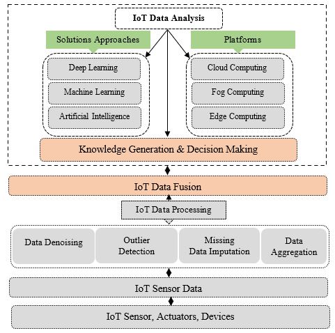
Figure 1: The basic architecture for IoT sensor data processing, data fusion and data analysis
FIGURE 2
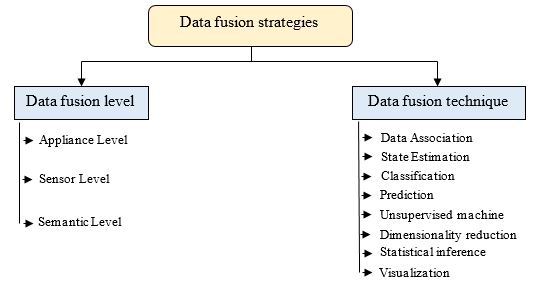
Figure 2: Taxonomy of data fusion strategies
FIGURE 3
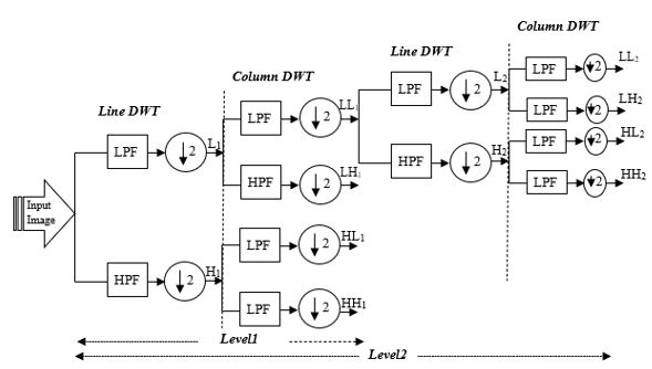
Figure 3: Two-level decomposition algorithm for 2-D DWT
FIGURE 4
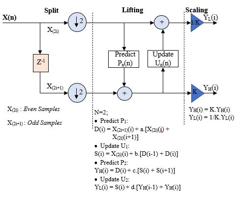
Figure 4: The implementation of the 1D-DWT lifting scheme
FIGURE 5
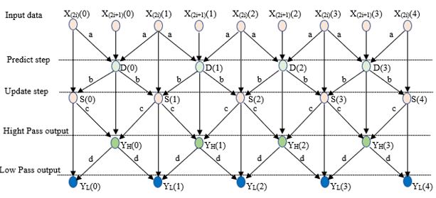
Figure 5: The schematic of 1-D DWT using lifting scheme for (9, 7) filter
FIGURE 6
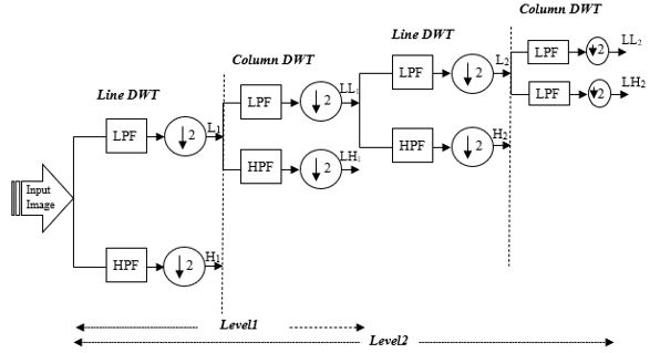
Figure 6: Two-level decomposition algorithm for SHPS technique
FIGURE 7
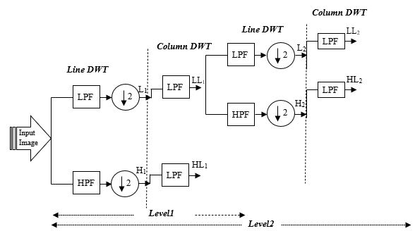
Figure 7: Two-level decomposition algorithm for EHPF technique
FIGURE 8
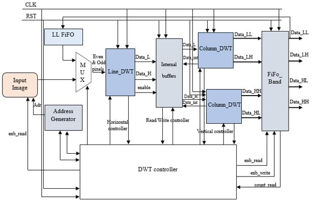
Figure 8: The block diagram of the proposed 2D-DWT architecture
FIGURE 9
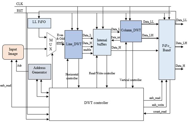
Figure 9: The block diagram of the proposed SHPS architecture.
FIGURE 10
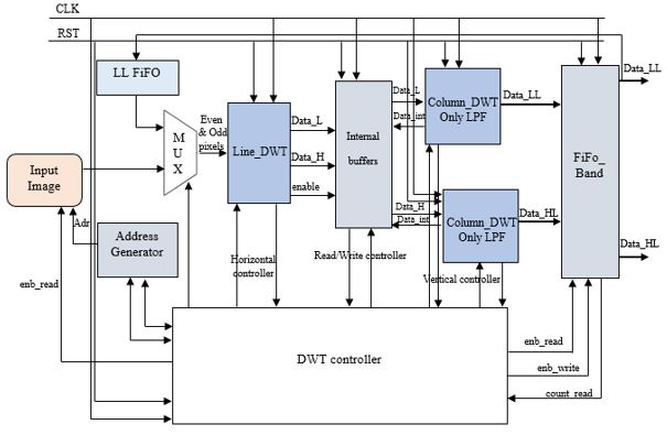
Figure 10: The block diagram of the proposed EHPF architecture
FIGURE 11
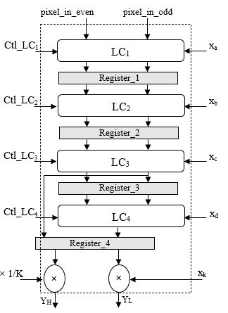
Figure 11: 1D-DWT architecture block diagram
FIGURE 12
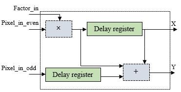
Figure 12: Each Lifting Computation's basic architecture
FIGURE 13
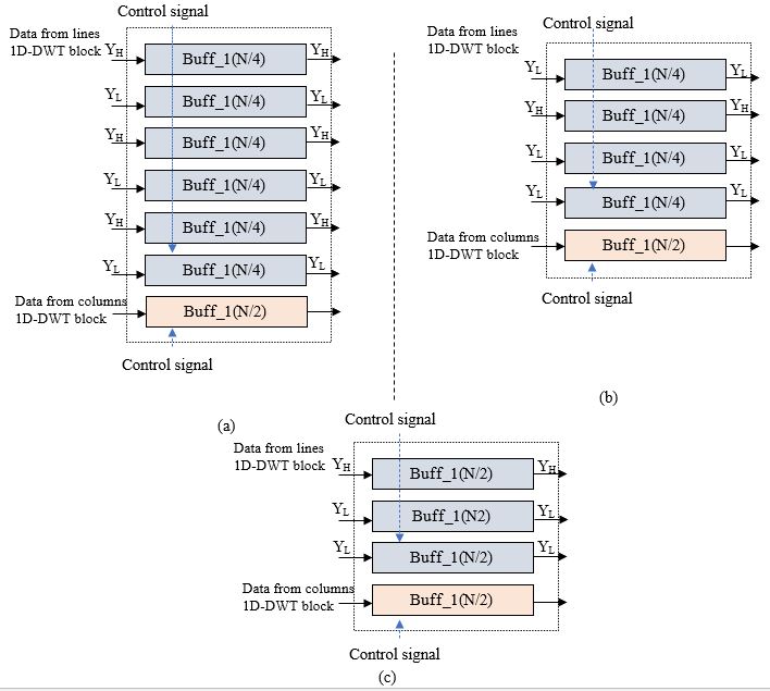
Figure 13: Internal buffers structure for: (a) (9, 7) filter; (b) SHPS technique; (c) EHPF technique
FIGURE 14
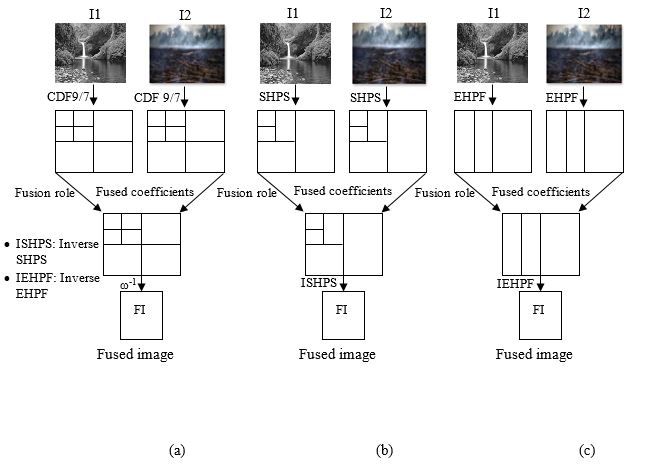
Figure 14: 14: Schematic Diagram of Image Fusion. (a) Image Fusion-based DWT; (b) Image Fusion-based SHPS; (c) Image Fusion-based EHPF
FIGURE 15
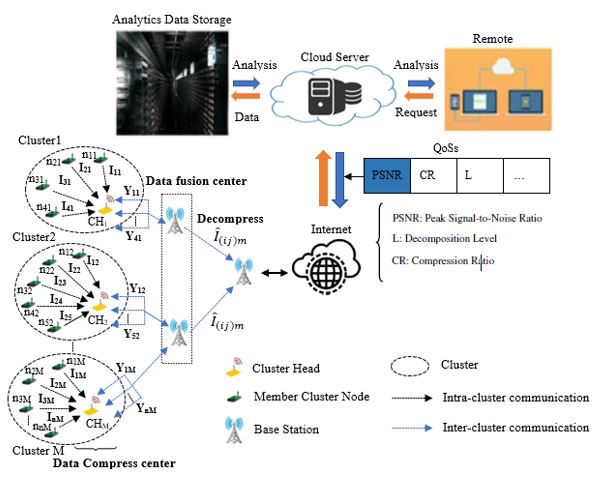
Figure 15: The intelligent monitoring system-based approach
FIGURE 16
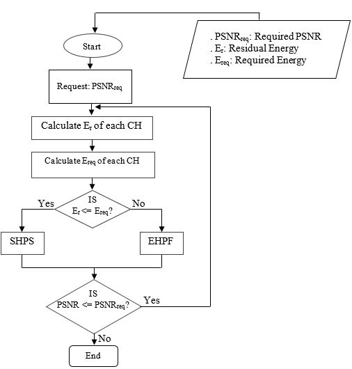
Figure 16: Flowchart of EEWIFT
FIGURE 17
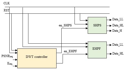
Figure 17: The block diagram of the proposed EEWIFT
FIGURE 18
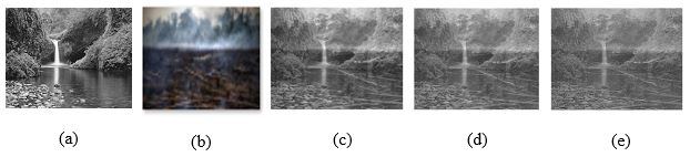
Figure 18: Visual results of fused image. (a) Input source image1 (b) Input source image2 (c) CDF 9/7-based fusion: PSNR= 16.52 dB; (d) EHPF-based fusion: PSNR = 13.88 dB; (e) SHPS-based fusion: PSNR= 12 dB
FIGURE 19
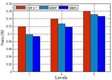
Figure 19: Power consumption comparison between CDF 9/7 DWT and proposed approaches
Tables at a glance
Figures at a glance